Figure 1: Hyperparameter tuning problem with a 2D search space. Each point represents a specific hyperparameter configuration and warmer colors correspond to better performance. Notice that adaptive selection methods for hyperparameter tuning proceed sequentially and concentrate on promising regions of the search space.
Machine learning algorithms typically have configuration parameters, or hyperparameters, that influence their output and ultimately predictive accuracy (Melis et al., 2018). Some common examples of hyperparameters include learning rate, dropout, and activation function for neural networks, maximum tree depth for random forests, and regularization rate for regularized linear regression.
In practice, applying machine learning solutions requires carefully tuning the hyperparameters pertaining to the model in order to achieve high predictive accuracy. Certain problems like reinforcement learning and GAN training are notoriously hard to train and highly sensitive to hyperparameters (Jaderberg et al., 2017; Roth et al., 2017). In other instances, hyperparameter tuning can drastically improve the performance of a model, e.g., carefully tuning the hyperparameters for an LSTM language model beat out many recently proposed recurrent architectures that claimed to be state-of-the-art (Melis et al, 2018; Merity et al., 2017 ).
Practitioners often tune these hyperparameters manually (i.e., graduate student decent) or default to brute-force methods like systematically searching a grid of hyperparameters (grid search) or randomly sampling hyperparameters (random search), both of which are depicted in Figure 1. In response, the field of hyperparameter optimization addresses the important problem of automating the search for a good hyperparameter configuration quickly and efficiently.
A new paradigm in hyperparameter optimization
In the current era of machine learning, learning algorithms often contain half-a-dozen hyperparameters (and easily more) and training a single model can take days or weeks rather than minutes or hours. It is simply not feasible to train several models sequentially and wait days, weeks or months to finally choose a model to deploy. In fact, a model may need to be selected in roughly the same wall-clock time needed to train and evaluate only a single hyperparameter configuration. In such a setting, we need to exploit parallelism to have any hope of finding a good configuration in a reasonable time. Luckily, the increased prevalence of cloud computing provides easy access to distributed computing resources and scaling up hyperparameter search to more machines isfeasible. We argue that tuning computationally heavy models using massive parallelism is the new paradigm for hyperparameter optimization.
Many existing methods for hyperparameter optimization use information from previously trained configurations to inform which hyperparameters to train next (see Figure 1, right). This approach makes sense when models take minutes or hours to train: waiting a few rounds to learn which hyperparameters configurations are more likely to succeed still allows a reasonable window for feedback and iteration. If a machine learning problem fits into this paradigm, using these sequential adaptive hyperparameter selection approaches can provide significant speedups over random search and grid search. However, these methods are difficult to parallelize and generally do not scale well with the number workers.
In the parallel setting, practitioners default to using random and grid search for hyperparameter optimization in the parallel setting because the two methods are trivial to parallelize and easily scale to any number of machines. However, both methods are brute force approaches that scale poorly with the number of hyperparameters. The challenge going forward is how to tackle increasingly more complex hyperparameter optimization tasks with higher dimensions that push the limits of our distributed resources. We propose addressing this challenge with an asynchronous early-stopping approach based on the successive halving algorithm.
Principled early-stopping with Successive Halving
Recently we proposed an algorithm that uses the successive halving algorithm (SHA), a well-known multi-armed bandit algorithm, to perform principled early stopping. The successive halving algorithm begins with all candidate configurations in the base rung and proceeds as follows:
- Uniformly allocate a budget to a set of candidate hyperparameter configurations in a given rung.
- Evaluate the performance of all candidate configurations.
- Promote the top half of candidate configurations to the next rung.
- Double the budget per configuration for the next rung and repeat until one configurations remains.
The algorithm can be generalized to allow for a variable rate of elimination η so that only 1/η of configurations are promoted to the next rung. Hence, higher η indicates a more aggressive rate of elimination where all but the top 1/η of configurations are eliminated.
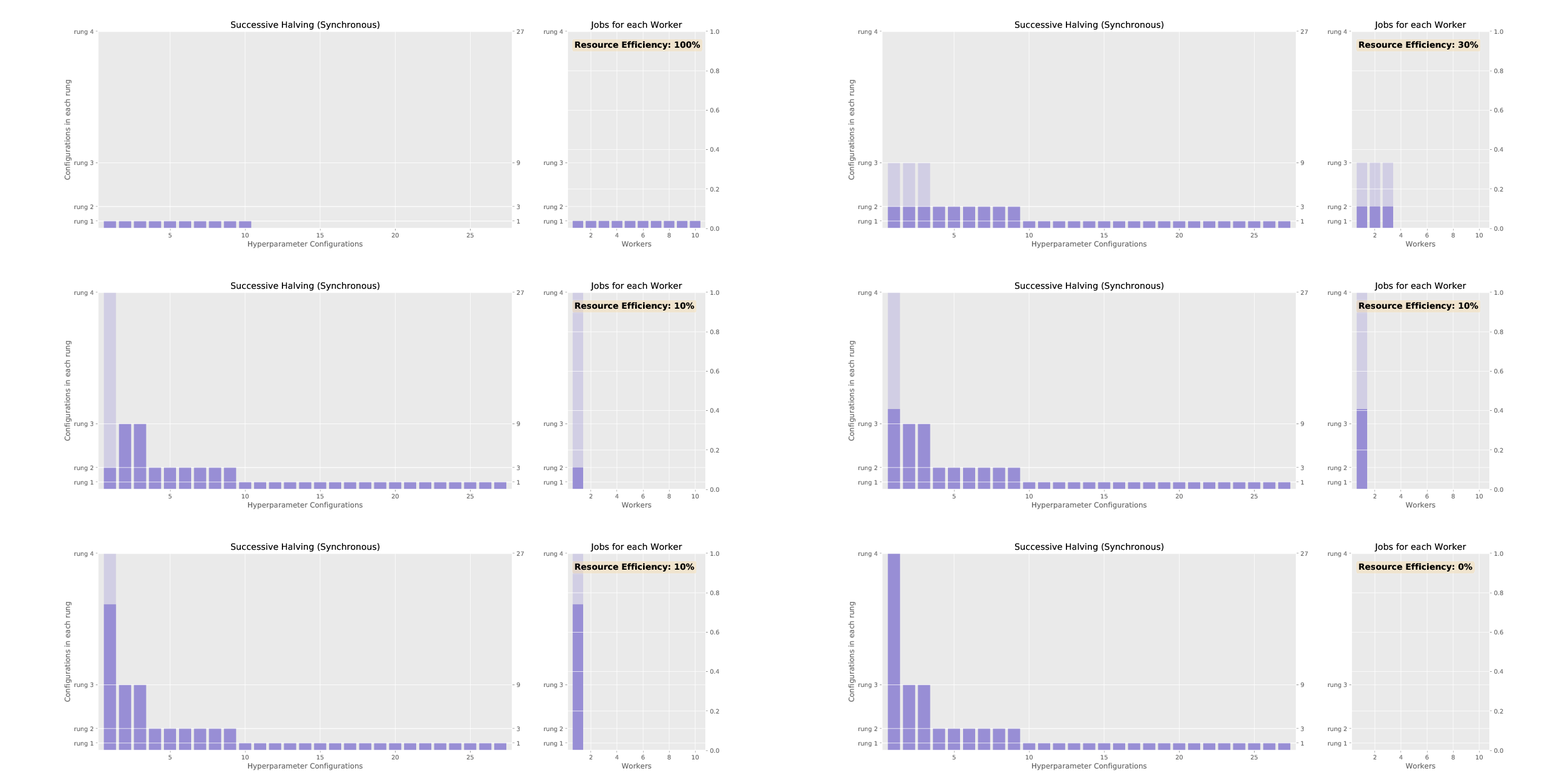
To demonstrate SHA, consider the problem of tuning a grid of 3 hyperparameters for a 2 layer neural network: learning rate (0.1, 0.01, 0.001), momentum (0.85, 0.9, 0.95), and weight decay (0.01, 0.001, 0.0001). This allows for a total of 27 different hyperparameter configurations. In the table below, we show the rungs for SHA run with 27 configurations, a minimum resource per configuration of 1 epoch, and a rate of elimination 3. The synchronized promotions of SHA according to the schedule shown in the table is animated in Figure 2.
| Configurations Remaining | Epochs per Configuration |
| Rung 1 | 27 | 1 |
| Rung 2 | 9 | 3 |
| Rung 3 | 3 | 9 |
| Rung 4 | 1 | 27 |
Table 1: SHA with η=3 starting with 27 configurations, each allocated a resource of 1 epoch in the first rung.
Asynchronous Successive Halving for the parallel setting
In the sequential setting, successive halving evaluates orders of magnitude more hyperparameter configurations than random search by adaptively allocating resources to promising configurations. Unfortunately, it is difficult to parallelize because the algorithm takes a set of configurations as input and waits for all configurations in a rung to complete before promoting configurations to the next rung.
To remove the bottleneck created by synchronous promotions, we tweak the successive halving algorithm to grow from the bottom up and promote configurations whenever possible instead of starting with a wide set of configurations and narrowing down. We call this the Asynchronous Successive Halving Algorithm (ASHA).
ASHA begins by assigning workers to add configurations to the bottom rung. When a worker finishes a job and requests a new one, we look at the rungs from top to bottom to see if there are configurations in the top 1/η of each rung that can be promoted to the next rung. If not we assign the worker to add a configuration to the lowest rung to grow the width of the level so that more configurations can be promoted.
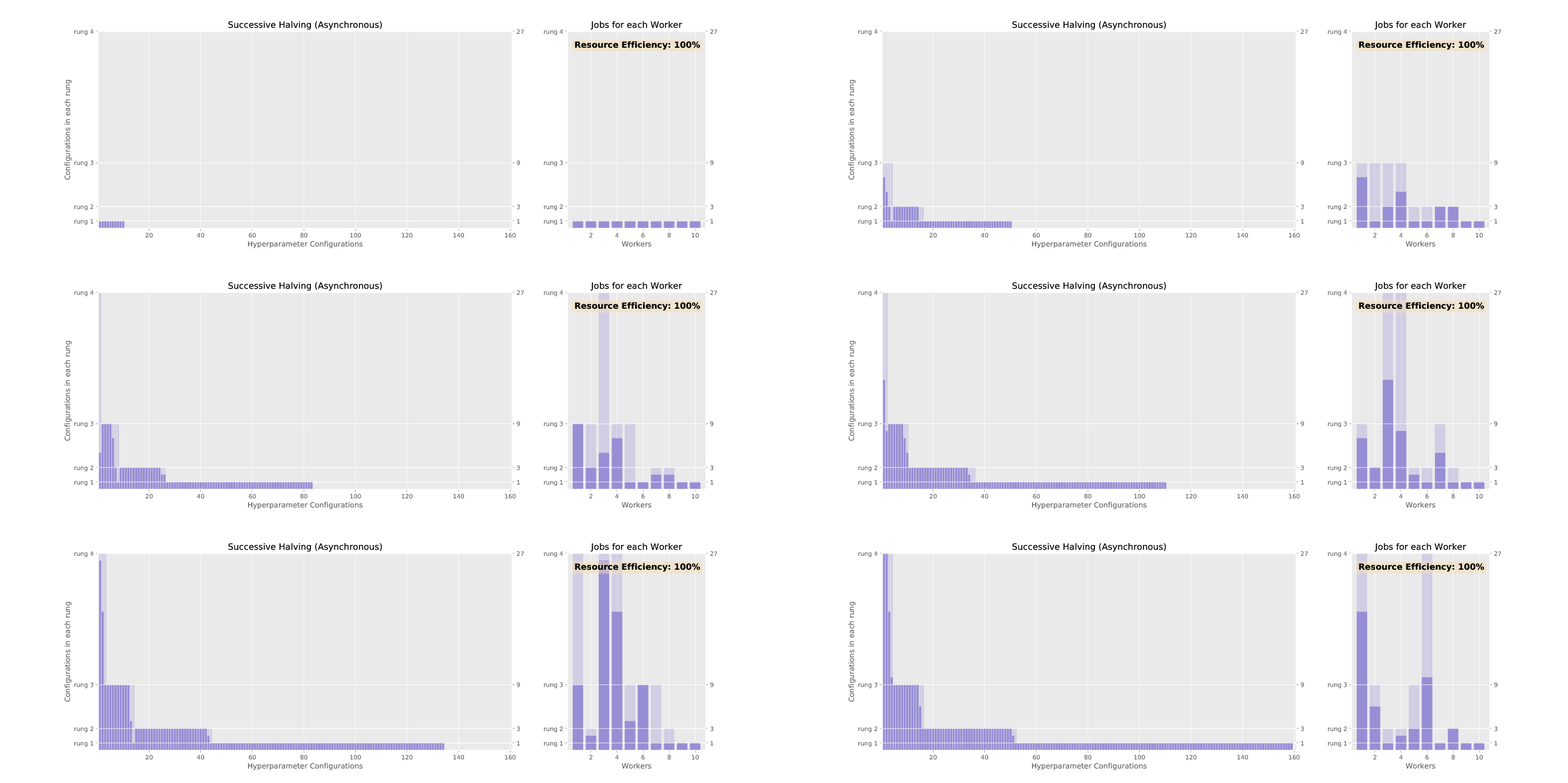
Figure 2 and 3 animate the associated promotion schemes for synchronous and asynchronous successive halving when using 10 workers and the associated worker efficiency for each. As shown in Figure 2, the naive way of parallelizing SHA, where each configuration in a rung is distributed across workers, diminishes in efficiency as the number of jobs dwindle for higher rungs. In contrast, asynchronous SHA approaches near 100% resource efficiency as workers are always able to stay busy by expanding the base rung if no configurations can be promoted to higher rungs.

Figure 2: Successive halving with synchronous promotions.

Figure 3: Successive halving with asynchronous promotions.
Results on small-scale benchmarks
In our first set of experiments, we compare ASHA to SHA and PTB on two benchmark tasks on CIFAR-10: (1) tuning a convolutional neural network (CNN) with the cuda-convnet architecture and the same search space as Li et al. (2017); and (2) tuning a CNN architecture with varying number of layers, batch size, and number of filters. PTB is a state-of-the-art evolutionary method that iteratively improves the fitness of a population of configurations after partially training the current population. For a more extensive comparison of ASHA to additional state-of-the-art hyperparameter optimization methods, please take a look at our full paper.
The resources allocated to the rungs as a fraction of the maximum resource per model R by SHA and ASHA are shown in Table 2; the number of remaining configurations in synchronous SHA is shown as well. Note that we use an elimination rate of η=4 so that only the top ¼ of configurations are promoted to the next rung.
| Configurations Remaining | Epochs per Configuration |
| Rung 1 | 256 | R/256 |
| Rung 2 | 64 | R/64 |
| Rung 3 | 16 | R/16 |
| Rung 4 | 4 | R/4 |
| Rung 5 | 1 | R |
Table 2: SHA with η=4 starting with 256 configurations, each allocated a resource of R/256 in the first rung. ASHA simply allocates the indicated resource to configurations in each rung and promotes configurations in the top 1/4th to the rung above.
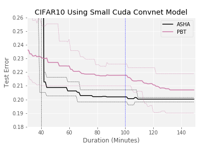
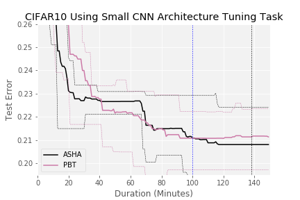
We compare the methods in both single machine and distributed settings. Figure 4 shows the performance of each search method on a single machine. Our results show that SHA and ASHA outperform PTB on the first benchmark and all three methods perform comparably in the second. Note that ASHA achieves comparable performance to SHA on both benchmarks despite promoting configurations asynchronously.
Figure 4: Comparison of hyperparameter optimization methods on 2 benchmark tasks using a single machine. Average across 10 trials is shown with dashed lines representing top and bottom quintiles.
As shown in Figure 5, the story is similar in the distributed setting with 25 workers. For benchmark 1, ASHA evaluated over 1000 configurations in just over 40 minutes with 25 workers (compared to 25 for random search) and found a good configuration (error rate below 0.21) in approximately the time needed to train a single model, whereas it took ASHA nearly 400 minutes to do so in the sequential setting (Figure 4). Notably, we only achieve a 10× speedup on 25 workers due to the relative simplicity of this task, i.e., it only required evaluating a few hundred configurations before identifying a good one in the sequential setting. In contrast, when considering the more difficult search space in benchmark 2, we observe linear speedups with ASHA, as the roughly 700 minutes in the sequential setting (Figure 4) needed to find a configuration with test error below 0.23 is reduced to under 25 minutes in the distributed setting.
We further note that ASHA outperforms PBT on benchmark 1; in fact the minimum and maximum range for ASHA across 5 trials does not overlap with the average for PBT. On benchmark 2, PBT slightly outperforms asynchronous Hyperband and performs comparably to ASHA. However, note that the ranges for the searchers share large overlap and the result is likely not significant. ASHA’s slight outperformance of PBT on these two tasks, coupled with the fact that it is a more principled and general approach (e.g., agnostic to resource type and robust to hyperparameters that change the size of the model), further motivates its use for distributed hyperparameter optimization.


Figure 5: Comparison of hyperparameter optimization methods on 2 benchmarks using 25 machines. Average across 5 trials is shown with dashed lines representing min/max ranges. Black vertical dotted lines represent maximum time needed to train a configuration in the search space. Blue vertical dotted line indicates time given to each searcher in the single machine experiments in Figure 4.
Results on a large-scale hyperparameter optimization task
We tune a one layer LSTM language model for next word prediction on the Penn Treebank (PTB) dataset. Each tuner is given 500 workers to tune 9 different hyperparameters that control the optimization routine and the model architecture. We evaluate the performance of ASHA and compare to the default tuning method in Vizier, Google’s internal hyperparameter optimizer service, with and without early-stopping.
Our results in Figure 6 show that ASHA is 3x faster than Vizier at finding a good configuration; namely, ASHA is able to find a configuration with perplexity below 80 in the time it takes to train an average configuration for R resource (this search space contains hyperparameters that affect the training time like number of hidden units and batch size), compared to the nearly 3R needed by Vizier.
Figure 6: Large-scale ASHA benchmark that takes on the order of weeks to run with 500 workers. The x-axis is measured in units of average time to train a single configuration for R resource. The average across 5 trials is shown, with dashed lines indicating min/max ranges.
Notably, we observe that certain hyperparameter configurations in this benchmark induce perplexities that are orders of magnitude larger than the average case perplexity. Model-based methods that make assumptions on the data distribution, such as Vizier, can degrade in performance without further care to adjust this signal. We attempted to alleviate this by capping perplexity scores at 1000 but this still significantly hampered the performance of Vizier. We view robustness to these types of scenarios as an additional benefit of ASHA and Hyperband.
Where should I look next to learn more?
For more details about the successive halving algorithm and how we guarantee that the algorithm will not eliminate good configurations prematurely, see our original paper for the sequential setting. Finally, we refer interested readers to this paper for more details about the asynchronous version of the successive halving algorithm, an extended related work section, and more extensive empirical studies.
DISCLAIMER: All opinions expressed in this posts are those of the author and do not represent the views of CMU.