Why did a Deep Neural Network (DNN) make a certain prediction? Although DNNs have been shown to be extremely accurate predictors in a range of domains, they are still largely black-box functions—even to the experts who train them—due to their complicated structure with compositions of multiple layers of nonlinearities. The most popular approach used to shed light on the predictions of DNNs is to create what is known as a saliency map, which provides a relevance score for each feature. While saliency maps may provide insights on what features are important to a DNN, it remains unclear if or how to use this information to improve a given model. One potential solution is to show not only the set of features important to a DNN for some specific prediction, but also the most relevant set of training examples, i.e., prototypes. As we will show, these not only help us understand the predictions of a given DNN, but also provide insights into how to improve the performance of the model.
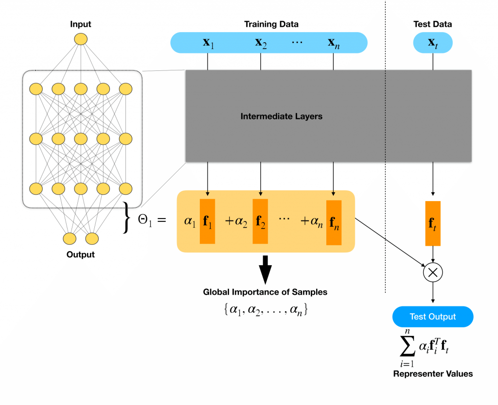
In our recent paper at NeurIPS 2018, we explain the prediction of a DNN by splitting the output into a sum of contributions from each of the training instances. Before getting into the formal details, here is an illustration of how our approach works for a DNN f and a similarity function K with some precalculated sample importance.
In the figure above, we consider an image classifier trained to determine whether an image is a dog or not, and the classifier is given an image of a dog (left) and a cat (right) at test time. To understand why the model predicted the first image as a dog and the second image as not a dog, we decompose the prediction score for the dog class (0.7 and 0 respectively) into a sum of the weighted similarities between the test image and each training image. This sheds light on which training images are most important for the prediction: the blue box highlights an example with high positive influence (which we call positive prototypes), and the red box highlights one with high negative influence (negative prototypes).
A Representer Theorem for Explaining Neural Networks
The idea of decomposing a predictor into a linear combination of functions of training points is not new (for interested readers, we refer you to representer theorems when the predictor lies in certain well-behaved spaces of functions). In the following theorem, we provide an analogous decomposition for deep neural networks.
Representer Theorem for Neural Networks: Let us denote the neural network prediction function of some testing input \(x_t\) by \(\hat{y_t} = \sigma(\Phi(x_t, \Theta))\), where \(\Phi(x_t, \Theta) = \Theta_1 f_t\) and \(f_t = \Phi_2(x_t,\Theta_2)\). In simple words, \(\sigma\) is the activation function over the output logit \(\Phi\), and \(\Theta_1\) is the weight of last layer which gets \(f_t\) as the input. Suppose \(\Theta^*\) is a stationary point of the optimization problem: \begin{equation} \arg\min_{\Theta} \{\frac{1}{n}\sum_i^n L(x_i,y_i,\Theta)) + g(||\Theta_1||)\},\end{equation} where \(g(||\Theta_1||) = \lambda ||\Theta_1||^2\) for some \(\lambda >0\). Then we have the decomposition: \begin{equation}\Phi(x_t,\Theta^*) = \sum_i^n \alpha_i k(x_t, x_i),\end{equation} where \(\alpha_{i} = \frac{1}{-2 \lambda n} \frac{\partial L(x_i,y_i,\Theta)}{\partial \Phi(x_i,\Theta)} \), \(k(x_t,x_i) = f_{i}^T f_t, \Theta^*_1 = \sum_i^n \alpha_i f_{i} \), and we call each term in the summation a representer value for \(x_i\) given \(x_t\). Also we will call each \(x_i\) associated with the representer value \(\alpha_i k(x_t, x_i)\) as a representer point. We note that \(\alpha_{i}\) measures the importance of the training instance \(x_i\) on the learned parameter, and thus we call \(\alpha_{i}\) the global sample importance since it is independent of the testing instance.
Our theorem indicates that the predictions of a deep neural network can be decomposed according to the figure below.
 We can decompose the weights of the final fully-connected layer of the neural network into a linear combination of feature maps for each training data (large orange box). Then given a test point, we can decompose the test output as a summation of the representer values.
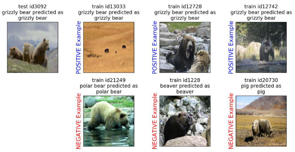
 Intuition for the Representer Theorem and examples of prototypes: For the representer value \(\alpha_i k(x_t, x_i)\) to be positive, we must have both global sample importance and the feature similarity to have the same sign. For a particular test image, this means that both the test image and training image look similar to each other, and (likely) have the same classification label. Similarly, for this value to be negative, the global sample importance and the feature similarity should have different signs e.g. one is negative and the other is positive. For a particular test image, this means that the images may look similar to each other, but they have different classification labels. Because we have decomposed the activation of the neural network into a sum of these representer values, we say that positive prototypes excite the network, and negative prototypes inhibit the network towards predicting a particular class.

As shown in the above figure, the positive representer points are all from the same class as the test point, and have a similar appearance. On the other hand, negative representer points belong to different classes despite their striking similarity in appearance.
Experiments
We demonstrate the usefulness of our representer points via two use cases:
- Misclassification Analysis
- Dataset Debugging
Then we wrap up with a discussion of the computational cost associated with our approach.
Misclassification Analysis
Why did the model mis-classify certain instances?
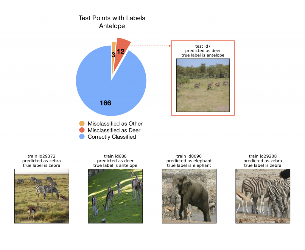
We want to use our class of explanations to understand the mistakes made by the model. With a Resnet-50 model trained on the Animals with Attributes (AwA) dataset (Xian et al. 2018), we pick test points with the ground-truth label “Antelope,” and analyze why the model made mistakes on some of these test points. Among 181 test instances labeled “Antelope”, 166 were classified correctly by the model, and 15 were misclassified. Among those 15, 12 were specifically misclassified as “Deer”, just as in the image shown below.
 Why is the image of the antelope predicted as deer? Because some training images that contain small antelopes with other animals are not labeled as antelopes but as a different class.
We computed representer points for all 12 of these misclassified test instances, and identified the top negative representer points for the class “Antelope.” Recall from the previous section that the top negative representer points are training points that inhibit the network from predicting “Antelope”, which can be used to make sense of why such inhibition occurred. For all 12 instances, the four representer points shown in the above figure (bottom row) were included among the top 5 negative representer points. Notice that these negative images do contain antelopes but have dataset labels belonging to different classes, like zebra or elephant. When the model is trained on these data points, the label forces the model to focus on just the elephant or zebra and ignore the antelope coexisting in the image. The model thus learns to inhibit the “Antelope” class given an image with small antelopes and other large objects. Hence, the representer points can point back to the errors in the training data that affected the model’s test-time prediction value.
Dataset Debugging
Given a training dataset with corrupted labels, can we correct the dataset? And can we achieve better test accuracy with the corrected dataset?
We consider a scenario where humans need to inspect the dataset quality to ensure an improvement of the model’s performance on the test data. Real-world data is bound to be noisy, and the bigger the dataset becomes, the more difficult it will be for humans to look for and fix mislabeled data points. Consequently, it is crucial to know which data points are more important than others to the model so that we can prioritize data points to inspect and facilitate the debugging process.
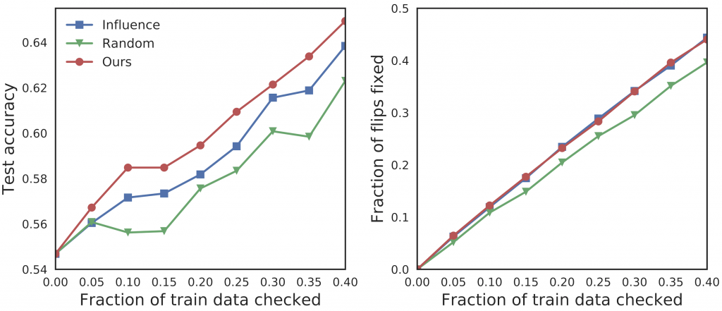
We run a simulated experiment where we check a fraction of the training data according to the order set by different importance scores, flip their labels, and retrain the model using the modified training data to observe the improvement of the test accuracy. We also evaluate how quickly different methods can recover and correct wrongly labeled data.

We used a logistic regression model for a binary classification task on the classes automobile vs horse from the CIFAR10 dataset. We used three methods to compute the importance values.
- Random (green line): randomly select the training point to fix.
- Influence function (blue line): select the training point with largest influence function value (Koh et al. 2017).
- Representer values (red line): select the training point with largest absolute global importance.
Our method recovers the test accuracy most quickly, and achieves comparable performance on correcting the right data points against the influence functions.
Computational Cost
All this is great, but can you compute these explanations quickly?
One advantage of our representer theorem is that it explicitly deconstructs a given deep neural network prediction in terms of representer values, so that we were able to achieve an orders of magnitude speedup compared to influence functions (even with a fine-tuning step that we require where we search for a stationary point, and which the influence function does not). Below shows the time in seconds for both methods to explain one testing instance in two different datasets.
Where should I look to learn more?
For more details on some theoretical aspects, as well as some additional experiments, please refer to the paper. We also encourage interested readers to try out our code on Github.
DISCLAIMER: All opinions expressed in this post are those of the author and do not represent the views of CMU.