Figure 1: Visualization of supervised neighborhoods for local explanation with MAPLE. When seeing the new point \(X = (1, 0, 1)\), this tree determines that \(X_2\) and \(X_6\) are its neighbors and gives them weight 1 and gives all other points weight 0. MAPLE averages these weights across all the trees in the ensemble.
Machine learning is increasingly used to make critical decisions such as a doctor’s diagnosis, a biologist’s experimental design, and a lender’s loan decision. In these areas, mistakes can be the difference between life and death, can lead to wasted time and money, and can have serious legal consequences.
Because of the serious potential ramifications of using machine learning in these domains, it falls onto machine learning practitioners to ensure that their models are robust and to foster trust with the people who interact with their models. Broadly speaking, meeting these two goals is the objective of interpretability and is achieved by iteratively: explaining both global and local behavior of a model (increasing understanding), checking that these explanations make sense (developing trust), and fixing any identified problems (preventing bad failures).
Meeting these two goals is a very difficult task and interpretability faces many challenges, but we will be focusing on two in particular:
- The frequently observed accuracy-interpretability trade-off where more interpretable models are often less accurate. Both accuracy and interpretability are desirable properties, so we do not want to have to choose between them.
- The existence of multiple types of explanations that each have their own advantages and disadvantages. We want to be able to combine their strengths and minimize their weaknesses.
Our proposed method, MAPLE, couples classical local linear modeling techniques with a dual interpretation of tree ensembles (which aggregate the predictions of multiple decision trees), both as a supervised neighborhood approach and as a feature selection method (see Fig. 1). By doing this, we are able to slightly improve accuracy while producing multiple types of explanations.
Before diving into the technical details of MAPLE and how it works as an interpretability system (both for explaining its own predictions and for explaining the predictions of another model), we provide an overview and comparison of the main types of explanations.
The Main Types of Explanations
At a high level, there are three main types of explanations:
- Example-based. In the context of an individual prediction, it is natural to ask: Which points in the training set most closely resemble a test point or influenced its prediction? Example: The K neighbors used by K-Nearest Neighbors.
- Local. We may aim to understand an individual prediction by asking: If the input is changed slightly, how does the model’s prediction change? Example: LIME (Ribeiro et al. 2016) uses a local linear model to approximate the predictive model in a neighborhood around the point being explained.
- Global. To gain an understanding of a model’s overall behavior we can ask: What are the patterns underlying the model’s behavior? Example: Anchors (Ribeiro et al. 2018) finds a rule-based approximation of as much of the model as possible.
Example-based explanations are clearly distinct from the other two explanation types, as the former relies on sample data points and the latter two on features. Furthermore, local and global explanations themselves capture fundamentally different characteristics of the predictive model. To see this, consider the toy datasets in Fig. 2 generated from three univariate functions.

Figure 2: Toy datasets from left to right (a) Linear (b) Shifted Logistic (c) Step Function.
Generally, local explanations are better suited for modeling smooth continuous effects (Fig. 2a). For discontinuous effects (Fig. 2c) or effects that are very strong in a small region (Fig. 2b), local explanations either fail to detect the effect or make unusual predictions, depending on how the local neighborhood is defined (i.e., whether or not it is defined in a supervised manner, more on this in the ‘Supervised vs Unsupervised Neighborhood’ section). We will call such effects global patterns because they are difficult to detect or model with local explanations.
Conversely, global explanations are less effective at explaining continuous effects and more effective at explaining global patterns. This is because they tend to be rule-based models that use feature discretization or binning. This processing doesn’t lend itself easily to modeling continuous effects (you need many small steps to approximate a linear model well) but does lend itself towards modeling the abrupt changes around global patterns (because those effects create natural cut-offs for the feature discretization or binning).
Most real datasets have both continuous and discontinuous effects and, therefore, it is crucial to devise explanation systems that can capture, or are at least aware of, both types of effects.
Because local explanations are actionable for (they answer the question “what could I have done differently to get the desired outcome?”) and relevant to (it is not particularly helpful to a person to know how the model behaves for an entirely different person) the people impacted by machine learning systems, we focus on them for this work.
Creating Local Explanations
The goal of a local explanation, \(g\), is to approximate our learned model, \(f\), well across some neighborhood of the input space, \(N_x\). Naturally, this leads to the fidelity-metric: \(E_{x’ \sim N_x}[ (g(x’) – f(x’))^2]\). The choices of \(g\) and \(N_x\) are important and should often be problem specific. Similar to previous work, we assume that \(g\) is a linear function.

Figure 3: A simple way of generating a local explanation that is very similar to LIME. From left to right, 1) Start with a point that you want to explain, 2) Define a neighborhood around that point, 3) Sample points from that neighborhood, and 4) Fit a linear model to the model’s predictions at those sampled points
MAPLE: Modifying Tree Ensembles to get Local Explanations
MAPLE (Plumb et al. 2018) modifies tree ensembles to produce local explanations that are able to detect global patterns and to produce example-based explanations; these modifications are built on work from (A. Bloniarz et al. 2016) and (S. Kazemitabar et al. 2017). Importantly, we find that doing this typically improves the predictive accuracy of the model and that the resulting local explanations have high fidelity.
Model Formulation
At a high level, MAPLE uses the tree ensemble to identify which training points are most relevant to a new prediction and uses those points to fit a linear model that is used both to make a prediction and as a local explanation. We will now make this more precise.
Given training data \((x_i, y_i)\) for \(i= 1, \ldots, n\), we start by training an ensemble of trees on this data, \(T_i\) for \(i= 1, \ldots, K\). For a point \(x\), let \(T_k(x)\) be the index of the leaf node of \(T_k\) that contains \(x\). Suppose that we want to make a prediction at \(x\) and also give an explanation for that prediction.
To do this, we start by assigning a similarity weight to each training point, \(x_i\), based on how often the trees put \(x_i\) and \(x\) in the same leaf node. So we define \(w_i = \frac{1}{K} \sum_{j=1}^K \mathbb{I}[T_j(x_i) = T_j(x)]\). This is how MAPLE produces example-based explanations; training points with a larger \(w_i\) will be more relevant to the prediction/explanation at \(x\) than training points with smaller weights. An example of this process for a single tree is shown in Fig. 1.
To actually make a prediction/explanation, we solve the weighted linear regression problem \(\hat\beta_x = \text{argmin}_\beta \sum_{i=1}^n w_i (\beta^T x_i – y_i)^2\). Then MAPLE makes the prediction \(f_{MAPLE}(x) = \hat\beta_x^T x\) and gives the local explanation \(\hat\beta_x\). Because the \(w_i\) depend on the training data (i.e., the most relevant points depend on the labels \(y_i\)), we say that \(\hat\beta_x\) uses a supervised neighborhood.
Supervised vs Unsupervised Neighborhoods Local Explanations
When LIME defines its local explanations, it optimizes for the fidelity-metric with \(N_x\) set as a probability distribution centered on \(x\). So we say it uses an unsupervised neighborhood. As mentioned earlier, the behavior of local explanations around global patterns depends on whether or not they use a supervised or unsupervised neighborhood.
Why don’t unsupervised neighborhoods detect global patterns? Near a global pattern, an unsupervised neighborhood will sample points on either side of it. Consequently, if the explanation is linear, it will smooth the global pattern (i.e., fail to detect it). Importantly, the only indication that something might be awry is that the explanation will have lower fidelity.
Although sometimes this smoothing is a good enough approximation, it would be better if the explanation detected the global pattern. For example, if we interpret Fig. 2b as the probability of giving someone a loan as their income increases, we can see that smoothing the global effect causes the explanation to give overly optimistic advice.
How are supervised neighborhoods different? On the other hand, supervised neighborhoods will tend to sample points only on one side of the global pattern and consequently will not smooth it. For example, in Fig. 2c, MAPLE will predict a slope of zero at almost all points because the function is flat across each one of its three learned neighborhoods.
But this clearly is also not a desirable behavior since it would imply that this feature does not matter for the prediction. Consequently, we introduce a technique to determine if a coefficient is zero/small because it does not matter or if it is zero/small because it is near a global pattern.
We do this by examining the probability distribution over the features induced by the weights, \(w_i\), and training points, \(x_i\), and determining where the explanation can be applied. Note that this distribution is defined using the weights learned by MAPLE. When a point is near a global pattern, this distribution becomes skewed and we can detect it. A brief example is shown bellow in Fig. 4 (see the paper for complete details).

Figure 4: An example of the local neighborhoods learned by MAPLE as we perform a grid search across the active feature of each of the toy datasets from Fig. 2. Notice that we can detect the strong effect by the small neighborhood in the steep region of the logistic curve (middle) and the discontinuities in the step function (right).
In summary, by using the local training distribution that MAPLE learns around a point, we can determine whether or not that point is near a global pattern.
Results
When evaluating the effectiveness of MAPLE, there are three main questions:
- Do we sacrifice accuracy to gain interpretability?
- How well do its local explanations explain its own predictions?
- How well can it explain a black-box model?
We evaluated these questions on several UCI datasets [Dheeru 2017] and will summarize our results here (for full details, see the paper).
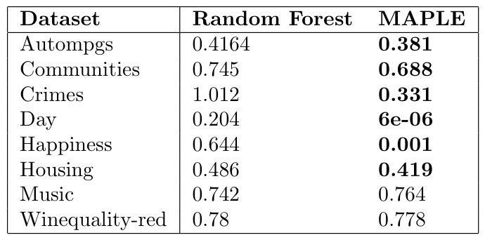
1. Do we sacrifice accuracy to gain interpretability? No, in fact MAPLE is almost always more accurate than the tree ensemble it is built on.
 Table 1: Comparing the Mean Squared Error of a Random Forest to MAPLE. Bold values indicate a significant difference (averaged over 50 trials).
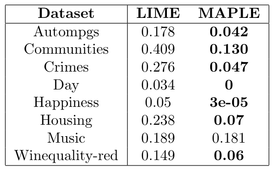
2. How well do its local explanations explain its own predictions? When comparing MAPLE’s local explanation to an explanation fit by LIME to explain the predictions made by MAPLE, MAPLE produces substantially better explanations (as measured by the fidelity metric).
 Table 2: Comparing the Fidelity Metric for MAPLE’s explanations of itself to LIME’s explanations of MAPLE. Bold values indicate a significant difference (averaged over 25 trials).
This is not surprising since this is asking MAPLE to explain itself, but it does indicate that MAPLE is an improvement on tree ensembles in terms of both accuracy and interpretability.
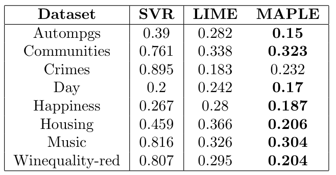
3. How well can it explain a black-box model? When we use MAPLE or LIME to explain a black-box model (in this case a Support Vector Regression model), MAPLE often produces better explanations (again, measured by the fidelity metric).
 Table 3: Comparing the Fidelity Metric for MAPLE’s explanations of a Support Vector Regression model to LIME’s explanations (SVR column is its mean squared error). Bold values indicate a significant difference (averaged over 25 trials).
Conclusion
By using leaf node membership as a form of supervised neighborhood selection, MAPLE is able to modify tree ensembles to be substantially more interpretable without the typical accuracy-interpretability trade-off. Additionally, it is able to provide feedback for all three types of explanations: local explanations via training a linear model, example-based explanations via highly weighted neighbors, and finally, detection of global patterns by using the supervised neighborhoods.
References
Marco Tulio Ribeiro, Sameer Singh, and Carlos Guestrin. “Why should i trust you?: Explaining the predictions of any classifier.” Proceedings of the 22nd ACM SIGKDD international conference on knowledge discovery and data mining. ACM, 2016.
Ribeiro, Marco Tulio, Sameer Singh, and Carlos Guestrin. “Anchors: High-precision model-agnostic explanations.” Thirty-Second AAAI Conference on Artificial Intelligence. 2018.
Gregory Plumb, Denali Molitor, and Ameet S. Talwalkar. “Model Agnostic Supervised Local Explanations.” Advances in Neural Information Processing Systems. 2018.
A. Bloniarz, C. Wu, B. Yu, A. Talwalkar. Supervised Neighborhoods for Distributed Nonparametric Regression. AISTATS, 2016.
S. Kazemitabar, A. Amini, A. Bloniarz, A. Talwalkar. Variable Importance Using Decision Trees. NIPS, 2017.
Dua Dheeru and Efi Karra Taniskidou. UCI machine learning repository, 2017.
DISCLAIMER: All opinions expressed in this post are those of the author and do not represent the views of CMU.