Figure 1: Interpretability for machine learning models bridges the concrete objectives models optimize for and the real-world (and less easy to define) desiderata that ML applications aim to achieve.
Introduction
The objectives machine learning models optimize for do not always reflect the actual desiderata of the task at hand. Interpretability in models allows us to evaluate their decisions and obtain information that the objective alone cannot confer. Interpretability takes many forms and can be difficult to define; we first explore general frameworks and sets of definitions in which model interpretability can be evaluated and compared (Lipton 2016, Doshi-Velez & Kim 2017). Next, we analyze several well-known examples of interpretability methods–LIME (Ribeiro et al. 2016), SHAP (Lundberg & Lee 2017), and convolutional neural network visualization (Olah et al. 2018)–in the context of this framework. Model interpretability has no absolutes and we discuss what these methods achieve as well as their limitations. We conclude by making general remarks about the field in light of these examples.
What is interpretability? (Lipton 2016, Doshi-Velez & Kim 2017)
Interpretability is difficult to define because models can be easy to understand in some aspects but not in others. The desired aspects in particular cases may also often be domain- or problem-specific, and while many papers have claimed interpretable models in various domains or applications, the machine learning community lacks a unifying framework for discussing what properties make a model interpretable and what we hope to do with interpretable results. Lipton (2016) presents such a framework under which we can discuss and compare the interpretability of models. In this paper, the author outlines both what we look to gain from interpretable ML systems as well as in what ways interpretability can be achieved. Similarly, Doshi-Velez & Kim (2017) outline a structured way to think about how interpretability methods can be evaluated.
When and why do we want interpretability?
Machine learning models are trained to optimize an objective function, which is often an accuracy-based metric. In many scenarios, an objective function cannot accurately capture the real-world costs of a model’s decisions. Costs related to ethics or fairness are difficult to specify in an objective function, and researchers may not know or be able to observe these costs a priori.
Interpretability is needed when model metrics are not enough. Interpretability allows us to understand what exactly a model is learning, what other information the model has to offer, and the justifications behind its decisions, and evaluate all of these in the context of the real-world problem we are trying to solve.
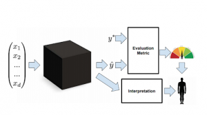
Figure 2: Stakeholders demand interpretability when the evaluation metric does not reflect the real cost of a model in deployment. The interpretation of the model and its decisions confer information about the true desiderata. (Lipton 2016)
What do we want from interpretability?
Trust: Interpretability can be defined as a prerequisite for humans to trust models. But just like interpretability, trust is difficult to define. One way to define trust is how comfortable we are with deploying the model in the real world. We might feel more at ease with a model that is better-understood, especially in high stakes decision making (e.g. finance or medicine), but this comfort does not necessarily reflect how accurate or effective a model is. In the case of trust, we care about where models make mistakes and not just how many. We especially desire that the model does not make mistakes where humans do not. Further, when the deployment environment diverges from the training environment, we look for confidence that the model will continue to perform well.
Causality: Supervised models learn associations between variables and outcomes, and are useful for generating hypotheses that scientists can then test in the real world. One example could be a learned relationship between thalidomide use and birth defects; upon discovering such an association in data, scientists could conduct a clinical trial to test if there is a cause-and-effect relationship.
Transferability: Humans possess a far greater ability to generalize than machine learning models do. Model interpretability helps us understand how models might fare when the test environment shifts from the training environment. In some cases, this shift is a natural consequence of the data itself, or as a result of the model deployment changing the environment itself. One example of models’ poor ability to generalize is adversarial attacks. Models are susceptible to such attacks and thus make mistakes that humans would never make. These adversarial attacks can have disastrous consequences when machine learning models such as facial recognition systems are deployed in the real world. Understanding how models work will help us be more aware of potential problems and guard against such possibilities.

Figure 3: The classic example of an adversarial attack that leads a convolutional neural network to classify a panda as a gibbon. Humans would never make the same mistake, and we need interpretability in models to be aware of and guard against such attacks. (Goodfellow 2015)
Informativeness: In many cases, the objective that the model is optimizing serves only as weak supervision for the real-world purpose of providing useful information to human decision-makers. The model uses the guidance provided by the objective to explore the data. Examples include intermediate features learned by convolutional networks and the magnitude of parameters in a linear regression model.
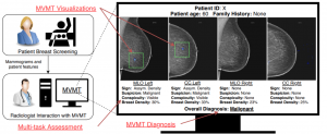
Figure 4: An example of informativeness from “Multi-view Multi-task Learning for Improving Autonomous Mammogram Diagnosis” (Kyono 2019). Here, an ML system outputs additional features for radiologists to scrutinize along with the final diagnosis, providing valuable information to assess why certain predictions were being made. As the neural network in the model learns the same radiological features that radiologists use for diagnosis, it can be much more telling than the final output of the network itself when provided to humans. (Kyono 2019)
Fair and Ethical Decision Making: To determine whether the decisions made by models conform to ethical standards, we must be able to interpret results. As a practical example, new regulations by the European Union proposed that individuals affected by algorithmic decisions have a right to an explanation. To allow this, algorithmic decisions must be explainable, contestable, and modifiable in the case that they are incorrect.
What are the properties of interpretable models?
Model interpretability falls under two broad categories: transparency and post-hoc explanations. In transparency, we aim to understand the mechanism by which the model works. In contrast, post-hoc explanations aim to extract information from trained models to elucidate what exactly they have learned.
Transparency can be divided into three levels, each referring to a different part of a model:
- Simulatibility: a human can take the inputs and go through the calculations of the model in a reasonable time
- Decomposability: each part of the model (inputs, parameters, calculation) has an intuitive explanation
- Algorithmic transparency: theoretical guarantees about the convergence or behavior of the algorithm
While transparent models can lend greater insight into their inner workings, restricting ourselves to this definition of transparency leads to several disadvantages. First, the very definition of transparency often restricts us to simple or compact models (e.g. linear models with interpretable inputs, not-so-deep decision trees). Deep networks, which are widely used in the ML community, clearly lack simulatibility as well as decomposability because parameters in the hidden layer do not have an intuitive explanation. For nonconvex problems, we also have no guarantee of convergence with stochastic gradient descent. Second, humans do not exhibit transparency nor do we require this form of transparency when we process each others’ thoughts and decisions. We may not know exactly what neural computations lead us to make a decision or cause us to learn something, but we can explain after the fact the logic or reasoning behind our thoughts. These explanations help us and others determine whether a decision or thought was fair, logical, or well-thought-out. This form of post-hoc explanation applies to model interpretability as well.
Post-hoc explanations are methods by which what models have learned can be visualized. Common examples are:
- Text explanations: Similar to how humans justify decisions verbally. An explanation- or text-generating model is trained in tandem with the prediction model.
- Visualization: Qualitative determination of how the model is learned. Examples include t-SNE or enhancing activations of nodes in hidden layers.
- Local explanations: Visualizes what a network depends on locally, which is useful when global explanations are difficult to produce succinctly. Examples include saliency maps.
- Explanation by example: Similar to how humans justify actions by analogy. Outputs nearest training examples in the latent representation learned by the model. Examples include k-nearest neighbors and learned representations of words after word2vec training.

Figure 5: An example of text explanations that can be used to interpret what a model has learned: captions generated in tandem with visual recognition tasks. (Karpathy 2015)
Post-hoc explanations can be useful for research and interpretability, but they should not be accepted blindly. While post-hoc explanations can increase understanding, comfort, and trust of a model, they are not always guaranteed to explain the true underlying mechanism by which a model works. For example, college admissions leaders may often cite publicly-accepted reasons such as “leadership qualities” or “diversity” for acceptance, the real underlying reason could be race or legacy (Lipton 2016). Understanding why models work may increase our comfort with using them but may serve no practical cause nor confer genuine knowledge about how the model works. Post-hoc explanations can be extremely useful, but it is possibly counterproductive to spend too many resources generating low-impact explanations for models purely for the sake of trust or comfort.
How are Interpretability methods evaluated?
Evaluation of standard ML tasks can often be boiled down into well-defined numerical metrics. However, defining measurement for interpretability can be quite challenging. As outlined previously, there exists a large variety of potential tasks, desiderata, and types of methods that could achieve them. At the end of the day, what is seemingly agreed upon is that interpretability requires having a human perspective: the explanations offered should be helpful by providing insight into a human towards achieving some task. In this sense, perhaps directly measuring changes in user performance on specific tasks before and after explanations are introduced would give the most definitive conclusions about interpretability. On the other hand, such specific evaluations are expensive and perhaps don’t generalize to other applications. Addressing this tension between the rigorousness of task-specific user evaluations and their costs, Doshi-Velez & Kim (2017) thus present the following classification of interpretability evaluation methods. Ranking from most specific to least specific:
- Application-Grounded Evaluation: User tests are performed with expert humans performing specific real-world tasks. This means the more abstract “real objective”, such as whether a model or interpretability system actually helps on a real-world task, can be directly evaluated in terms of some final idealized performance.
- Human-Grounded Evaluation: User tests are performed with humans and simplified tasks. This alleviates some of the time and resource costs of application-grounded evaluation, as the task-complexity decreases along with the difficulty in finding appropriate human subjects. Also, more abstract concepts can be tested for (eg. effectiveness of explanations under time constraints) as the system can be more controlled.
- Functionally-Grounded Evaluation: No human subjects are involved and instead, some proxy measure of interpretability (eg. sparsity, local fidelity) is measured for the method, preferably on several datasets or applications.
In practice, all levels of evaluation are important. What is appropriate depends both on context and the specific research claim being made. If a paper is specific to a particular application or creates a type of explanation that is very unique to a certain field, rigorous effort should be put into conducting proper user studies. If a paper is improving upon an interpretability method that already has documented user studies, functionally-grounded evaluation could become more appropriate. Finally, these levels of evaluation should mutually inform one another. For example, numerical metrics for functionally-grounded evaluation can shed light on which proxies are best for which applications. In the other direction, perhaps it is an end application that inspires a new functionally-grounded evaluation metric.
In the following sections, we introduce three interpretability methods and examine how they fit within the interpretability frameworks proposed by Liption (2016) and Doshi-Velez & Kim (2017).
LIME (Ribeiro et al. 2016)
The first of these methods is a method for post-hoc explanations called LIME (Local Interpretable Model-Agnostic Explanations) (Ribeiro et al. 2016). As its full name suggests, LIME trades-off being limited to local explanations with the flexibility to apply to any black-box model. That being said, as the authors argue (and show empirically), explaining individual predictions can still be very useful for practitioners in terms of sanity-checking, debugging, and gaining insights into a complex model. Further, global conclusions about a model can still be gained by collecting a set of multiple local explanations. Specifically for this use case, the authors also propose an efficient explanation selection method, called SP-LIME, which tries to pick a small yet representative set of explanations to efficiently describe the overall model.
What is LIME?
As for the algorithm itself, LIME is conceptually quite simple. Given an example, \(x\), LIME attempts to fit an interpretable model locally that is faithful to the output of the original model, \(f(x)\), in a neighborhood around \(x\). This explanation aims to be:
- Easy-to-understand: Uses both an interpretable local model (e.g. sparse linear model or decision tree) and operates on interpretable features (which may be different from the inputs to \(f(x)\), more on this later).
- Locally Faithful: Actually matches up with \(f(x)\) when input is close to \(x\)
- Model-Agnostic: Only requires black-box queries to \(f(x)\)
Once the form of the local model is chosen, LIME creates each explanation by fitting the local model not on the original training dataset \(D\), but on a newly sampled dataset \(D_x\), which is sampled by randomly perturbing \(x\) in the interpretable feature space. Additionally, a kernel or distance metric is defined in the interpretable feature space and is used to weight the different elements of \(D_x\) based upon how close they are to \(x\). Thus, LIME essentially trains a weighted sparse least squares regression on \(D_x\) where the weights come from the kernel function. This process can be roughly summed up in Figure 6.
One previously mentioned caveat that merits greater elucidation is the notion of the interpretable representation. That is, while the original model is defined on \(f:X \rightarrow Y\), thus requiring inputs \(x \in X\), the explanation model needs to operate on understandable features. That is, it would not be helpful even to have a sparse linear model with a single non-zero weight if the active feature itself is not understandable. Instead, there often exists a more natural interpretable representation for the same example. We call this space of features \(X’\) and thus the explanation is defined on \(g:X’ \rightarrow Y\).
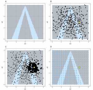
Figure 6: Panel A shows the decision boundary of \(f(x_1,x_2)\) B shows the prediction (yellow) being explained as well as the perturbation sampling step, C shows the neighborhood-based weighting of each sample, and D shows the explanation learned (white line) (Molnar 2019)
Two practical domains in which this distinction is important are when the inputs to \(f\) are images (ie. raw pixel values) or sentences (ie. in the form of word embeddings). In both cases, while these are sensible inputs for achieving good performance, they are difficult to parse by humans. Instead, a more interpretable representation for images would be the addition or removal of super-pixels. For the language case, a bag-of-words model that shows the presence and absence of individual tokens is more understandable.
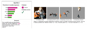
Figure 7: Examples of the interpretable feature representations for a language task (left) and image classification task (right), which are different from the features that would be fed to the original model (Ribeiro et al. 2016)
What desiderata does LIME attempt to address?
Along with the LIME algorithm itself, the authors in the original paper also largely position their work on the applicability of interpretable local models towards assessing trust. As they write, “Whether humans are directly using machine learning classifiers as tools, or are deploying models within other products, a vital concern remains: if the users do not trust a model or a prediction, they will not use it” (Ribeiro et al. 2016). To address these two general cases, the authors define two notions of trust:
- Trusting a Prediction: Can we make decisions based on a specific prediction?
- Trusting a Model: Can we deploy a model “in the wild” to perform well on real-world data according to the metrics of interest?
As such LIME directly aims to address the first notion of trust while it is argued that multiple single-prediction explanations can be combined to get a sense of trusting the model. At the same time, by allowing local explanations for any black-box model, the hope is to achieve a better trade-off between the predictive utility of ML models with explainability.
How does the LIME paper evaluate its claims?
Matching their motivating concern of trust, the LIME paper’s chief claims can be summarized as
- LIME (and SP-LIME) satisfy the desired properties for local explanations
- These local explanations have high utility in helping users reach the right conclusions/decisions about trusting models
To match these claims, they focus on human-grounded user studies (both simulated and real) for evaluating the utility of LIME explanations. That is, the “performance” of LIME is evaluated based upon how much it assists in a user’s actual ability to perform tasks. Focusing on the real-user experiments, the tasks are relatively simple and involve (1) choosing between a trustworthy and an untrustworthy model (2) helping improve an untrustworthy model via feature selection, and (3) detecting an irregularity in a classifier trained on a spurious correlation.
For (1), the authors train a classifier on documents about “Christianity” and “Atheism.” One version of the classifier is trained on the full original dataset, which suffers from data leakage: specific words and phrases are extremely predictive on the training and validation dataset but generalize poorly to a separate dataset also with articles about the two topics. The other version removes these problematic tokens, thus achieving worse validation accuracy but is more trustworthy. Here, users are shown 6 sparse linear explanations each with 6 weights and are asked to pick which model is preferred. Indeed, LIME explanations often show that these words that seemingly have nothing to do with religion indeed have high coefficients in the local models.
For (2), the authors start with the same untrustworthy model as in (1) and let the users progressively pick words to remove from the training set based upon the explanations they see. Indeed, they showed that even users who are not well-versed in ML can help improve the model considerably.
For (3), the authors train an image classifier trying to distinguish between huskies and wolves, a seemingly difficult problem. However, the training set leverages a spurious correlation in which all the photos with wolves have snow in the background. LIME explanations were able to identify these super-pixels as important factors in the decision and highlighted them to users. These users, who had at least taken an ML course, were then able to correctly identify the problem with the dataset.
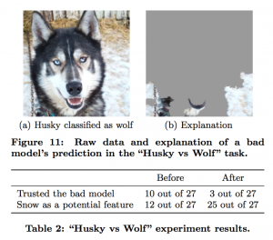
Figure 8: The results from the “Husky vs Wolf” experiments from the original LIME paper (Ribeiro et al. 2016). Displayed are an example of a LIME explanation on this dataset (top) as well as the results of the user study. In the first row of the table, users were asked to identify whether the bad model is trustworthy. In the second row, they were asked about their understanding of the model.
LIME within the Interpretability Framework
LIME is a very well-known and characteristic example of a post-hoc local explanation system. It tries to achieve the middle ground between allowing for a potentially complex underlying model (to not compromise on accuracy) with still providing useful explanations to individual predictions. While the authors focus on the issue of trust, their experiments also indicate that the local explanations created by LIME can also help assess and improve transferability. When explanations are paired with human prior knowledge, the paper shows that people can be guided towards choosing the right features for better generalization. For example, on both the Religions and the Husky vs. Wolf tasks, the core issue behind the lack of trust was that the “bad models” leveraged features that would lead to poor generalization.
Of course, this also comes with the potential pitfalls of post-hoc explanations, as put by Lipton:
“We caution against blindly embracing post-hoc notions of interpretability, especially when optimized to placate subjective demands. In such cases, one might deliberately or not, optimize an algorithm to present misleading but plausible explanations (Lipton 2016).”
Here, while the experiments were all positive indications of the potential utility of LIME explanations, they were designed to have very clean cut conclusions. That is, the authors chose setups where the failure of the “bad model” is quite simple and undiluted. In real applications, perhaps there could be multiple reasons that a model should not be trusted. As such, it would not necessarily be as easy to identify the correct issues, let alone would there be a guarantee that LIME achieves high local fidelity in the first place. In some sense, human intuition, which is biased in its own way, may overpower the uncertainty in the actual explanation. Explanations that “make sense” to a human may not actually describe the real model well and any conclusions made could be poor.
SHAP (Lundberg & Lee 2017)
We now we introduce SHAP (SHapley Additive exPlanations), a natural extension of LIME. To recap section 2, LIME introduces a framework for local, model-agnostic explanations using feature attribution. For any input \(x\) and model output \(f(x)\), LIME solves \(\xi(x) = \text{argmin}_{g \in G} L(f, g, \pi_x) + \Omega(g)\) to find an explanation \(g(x’) = \phi_0 + \sum \phi_i x’_i \), where \(g(x’) = f(x)\) (Lundberg & Lee 2017). Then, the \(i^{th}\) feature receives an attribution/importance score \(\phi_i\).
Desirable properties of explanations
However, LIME is just one possible way to solve for feature attribution scores, and not necessarily the best way. Let’s take a step back and consider three properties we want our explanations to have (Lundberg & Lee 2017).
- Local accuracy: If \(x’\) is the simplified \(x\), \(g(x’) = f(x)\).
- Missingness: “Missingness constrains features where \(x’_i = 0\) to have no attributed impact.” \(x’_i = 0 \Rightarrow \phi_i = 0\)
- Consistency: If a model changes so that feature \(i\) becomes more important, \(\phi_i\) should not decrease.
It turns out that most feature attribution methods ignore these three properties. For example, consider Gini importance, one of the default feature attribution methods in XGBoost.
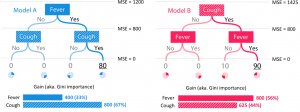
Figure 9: Misleading feature importance scores for two simple models as assigned by Gini importance. (Lundberg 2018)
Here, model A assigns a risk of 80 whenever fever and cough are both yes, and 0 otherwise. Model B is the same function, but with +10 risk whenever cough is yes. Intuitively, cough and fever are equally important in model A, while cough is more important than fever in model B, as removing it would more drastically change model B’s expected output and accuracy (Lundberg 2018). However, not only does model A assign unequal attributions to cough and fever, but model B gives more importance to fever than cough. In other words, due to its lack of consistency, Gini importance arguably gives poor explanations.
LIME has similar issues: while it always satisfies missingness, it can at times violate local accuracy and/or consistency. In fact, it turns out there is exactly one way to solve for feature attribution scores which satisfy local accuracy, missingness, and consistency: Shapley values (Lundberg & Lee 2017).
Shapley values
Shapley values were first developed by Lloyd Shapley to determine how to fairly split a payoff among players in a cooperative game (Wild 2018). Consider a game where Ashley, Ben, and Charles cooperate to win a cash prize by earning a payoff of 10 points. For example, they might answer 10 questions in a trivia game. You could think of Ashley joining the game first, then Ben, then Charles. When Charles joins, he may not be able to answer any questions that Ashley and Ben could not already answer, so his payoff should be $0. On the other hand, if Charles joined first, he might be able to answer 7 questions by himself, so his payoff should be 70% of the cash prize. Likewise, if Charles joins second after Ben, he might answer more questions than if he joins second after Ashley. As such, he might deserve a 40% payoff when joining after Ben, but only a 30% payoff when joining after Ashley.
The idea behind Shapley values is to average Charles’ marginal contributions over all possible orders in which he could have joined the game, and assign him that payoff. By considering features as players and the model output as the payoff, this exact idea can be applied to any machine learning model. Specifically, the Shapley value/feature attribution \(\phi_i\) for feature \(i\) can be calculated with the following equation: 
(Wild 2018)
Where \(F\) is the full feature set, \(f_S(x_S)\) is the model output with all features not in the current subset S set to 0, and \(f_{S \cup \{i\}}(x_{S \cup \{i\}})\) is the model output when you add feature \(i\) to \(S\).
Fast calculation, assumptions, and use cases of Shapley values
Unfortunately, calculating Shapley values using the above equation is computationally infeasible. However, Lundberg & Lee (2017) developed the SHAP package for faster calculation of Shapley values. Their first method, KernelExplainer, is a direct extension of LIME. It turns out that by appropriately modifying the LIME equation parameters, you can recover Shapley values:  Where \(|z’|\) is the number of non-zero elements in \(z’\).
Furthermore, the authors developed TreeExplainer, which calculates Shapley values for tree-based ensemble methods like XGBoost and LightGBM, as well as DeepExplainer, for deep neural networks. For example, in the case of image classification, DeepExplainer assigns a value to every pixel for every class, showing how that pixel influenced the model’s decision.

Figure 10: Red pixels (positive Shapley values) increase the model’s confidence in a class, blue pixels (negative Shapley values) decrease the model’s confidence, and clear pixels do not notably affect the model’s prediction. (Lundberg 2019)
Unfortunately, there are several disadvantages to SHAP. Since KernelExplainer makes many of the same assumptions as LIME, it has many of the problems discussed in section 2 (Budzik 2019). Moreover, KernelExplainer is often slower than LIME. Although DeepExplainer is faster than KernelExplainer, it can also be too slow to explain all instances in large datasets.
This makes SHAP’s most popular use case TreeExplainer, which trades the model-agnosticism of LIME and KernelExplainer for fast computation. With TreeExplainer, there is no need for an algorithm like SP-LIME to explain the best subset of a dataset. Instead, it is fast enough to compute Shapley values for entire datasets, which allows for global feature importance calculation. For example, you can average the magnitude of each Shapley value for any feature over an entire dataset, or you can plot the relationship between a feature’s Shapley value and its value (figure 11). Unfortunately, TreeExplainer often requires another assumption: to transform a model’s output non-linearly (such as converting a log-odds output to probability), it must assume that features are independent. This is a stringent assumption and can make using TreeExplainer inappropriate.
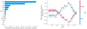
Figure 11: Left: Global feature importance scores calculated by averaging the magnitude of SHAP values over an entire dataset. Right: Scatterplot of Age SHAP values vs. Age value with interaction by sex. (Lundberg 2019)
SHAP within the interpretability framework
Beyond these assumptions, it is important to discuss what satisfying local accuracy, missingness, and consistency mean for interpretability as framed by Lipton (2016) and Doshi-Velez & Kim (2017). Even if its assumptions are satisfied, SHAP still only provides post-hoc explanations. We have no guarantee that these explanations faithfully reflect how the model is truly making its decision. Additionally, SHAP does not give us any better sense of algorithmic transparency or simulatability, and arguably no better explainability if the features themselves have been heavily engineered or transformed (though just as with LIME, SHAP can be applied to interpretable transformations on the input space like superpixels or word tokens).
On the other hand, SHAP helps with decomposability of the model: satisfying local accuracy, missingness, and consistency offers us higher confidence that the decomposed attributions given by SHAP are more accurate than those given by LIME. Indeed, for simple tasks like the sickness risk example from above or dividing out profit in a trivia game, SHAP aligns more closely with human intuition than LIME (figure 12). This human intuition comes from Amazon mechanical turk users, giving some proof that when evaluated on human-grounded metrics, with real humans and simplified tasks, SHAP outperforms LIME. Of course, this only suggests, but does not prove, SHAP will outperform LIME on application-grounded evaluation, with real-world tasks.

Figure 12: SHAP values align more closely with human intuition than LIME on simple tasks like assigning a sickness score from three features (A, 30 individuals) and assigning a payoff to each person in a 3-man team based on how many questions that person answered (B, 50 individuals). (Lundberg & Lee 2017)
SHAP and LIME are examples of post-hoc interpretation methods. While they may provide satisfying interpretations of a model’s decisions, they may not exactly elucidate the methods by which models work and can be potentially misleading. More direct visualization methods, an example of which is described in the next section, can reveal more about what exactly a model has learned.
The Building Blocks of Interpretability (Olah et al. 2018)
Pivoting away from separate explainer models proposed by LIME and SHAP, we now cover our last interpretability method: a method for extracting interpretability from convolutional neural networks presented in Olah et al. (2018). All information and images in this section were summarized and taken from the original paper, which can be viewed here. Thus far, most attempts at gleaning interpretability from CNNs have focused on the input and softmax layers. However, since most of the power of neural networks comes from the hidden layers, it seems natural to examine these hidden layers.
Visualizing individual neurons
At any hidden layer of a neural network, there are sets of vectors which can be viewed as activated neurons. Just as you can visualize an image from its pixel values, you can also visualize these neurons. Figure 13 shows one example, which visualizes the neurons across all channels of one location in the image and sorts the visualizations by their magnitude.
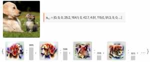
Figure 13: Visualizations of activated neurons, sorted by magnitude, for one location in an image, across the channels at one hidden layer of GoogLeNet. (Olah et al. 2018)
Clearly, these activated neurons have some useful interpretation. Though the visualizations aren’t images one might encounter in nature, they aren’t random noise either. The first two channels seem to be floppy ear and dog snout detectors, while the second two channels detect the pointy ears of a cat. Since the location in the image is the dog’s ear, these neurons having the highest magnitude is more than reasonable and provides insight that the model is making its decision in a way that corresponds to the human visual process.
Aggregating and visualizing neurons across channels
These base neurons can be aggregated in several ways (across channels, locations, layers), and the resulting aggregates can be visualized as well. For example, to get an overall idea for what the network is seeing at one point in an image in one hidden layer, you can weight each activated neuron by its magnitude, and sum across all channels.
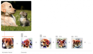
Figure 14: Visualization of neurons aggregated across all channels, for one location in an image, at one hidden layer of GoogLeNet. (Olah et al. 2018)
Though the aggregated neuron has a less clear interpretation than the individual neurons, it still informs on what the network sees while succinctly combining hundreds of neurons. For example, the aggregated neuron still resembles the floppy ears and snout of a dog – which makes sense, given which individual neurons had the highest magnitude. This aggregation is important; by applying this technique to all locations in an image, we can use one visualization to (relatively) efficiently summarize an entire hidden layer.
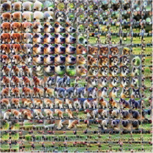
Figure 15: Visualization of all aggregated neurons for one hidden layer of GoogLeNet. (Olah et al. 2018)
As one would hope, the visualizations of the top-left of the image are clearly dog-like. Additionally, they are split into sections visualizing the dog’s head, ear, snout, and body. Similar visualizations are present for the part of the image that contains the cat. Again, they give us some confidence that the model is making decisions similar to how a human might (i.e. the model not only detects a dog and a cat, but splits them according to body parts). The sections of the image that contain grass are less structured, and one might expect them to be less useful for classification. Indeed, by scaling these aggregated neurons by their magnitudes and observing several hidden layers, you can see this is the case:

Figure 16: Visualization of all aggregated neurons for several hidden layers of GoogleNet, scaled by their magnitudes. (Olah et al. 2018)
Additionally, as the model goes deeper, it goes from attending to all parts of the image relatively equally to mainly attending to the sections containing the dog and cat, to focusing on the section with the dog. Once more, this process is in accord with human intuition.
Furthermore, we can combine the above image with feature attribution, by using saliency maps to background each aggregated neuron. Here, a saliency map is a simple heat map where red colors indicate neurons which encourage the model’s classification, blue colors indicate neurons which discourage the model’s classification, and grey neurons have minor effects.

Figure 17: Visualization of all scaled aggregated neurons for several hidden layers of GoogLeNet, with saliency maps. (Olah et al. 2018)
These saliency maps help confirm some implicit assumptions, and further validate the usefulness of the model. First, there is a high correlation between the magnitude of the aggregated neuron and the intensity of the saliency map. In other words, the areas in the image the model considers most important are actually the ones that most impact its decision. Second, the image of the dog correctly promotes the model’s labrador retriever classification, while the image of the cat correctly discourages it. This means the model isn’t just recognizing the structure of the animals in the image, but is differentiating between the dog and the cat.
Visualizing neurons across spatial locations
Thus far, we’ve focused on neurons aggregated over channels. Likewise, we can observe how each channel in different hidden layers, scanned over an entire image, contributes to the final classification.
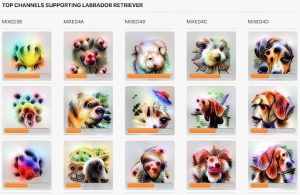
Figure 18: Visualization of the most useful channels at each hidden layer. (Olah et al. 2018)
As expected, channels deeper in the network pick up on more and more structure – the channels in mixed4c and mixed4d resemble dogs, while the lower layer channels are more abstract. Additionally, we observe that the most important filter for mixed4d captures more of a dog’s entire body than the filters we examined previously. Thus, it makes sense that it is the most important filter when the model considers the entire image, while the next two filters were more important when the model specifically examined the dog’s ear.
Condensing visualizations to human-scale
By aggregating over both channels and locations in the image, feature visualization and attribution give us powerful ways to interpret neural networks. Still, there is a trade-off: the most informative interpretation comes from considering both aggregation methods together, which is a lot of information. On the other hand, the aggregations we have already collected have lost much useful information – naively combining channel and spatial aggregations would lead to even more information loss. The goal then is to make interpretability human-scale by finding additional groupings of neurons which more effectively balance complexity and information retention.

Figure 19: Possible divisions of activated neurons. (Olah et al. 2018)
Importantly, the best neuron groupings depend on image content, and so vary from image to image. Therefore, universal splits such as image location or channel are no longer appropriate. Fortunately, this is a natural problem for matrix factorization. For example, by using non-negative matrix factorization, the top hidden layer of GoogLeNet for this specific image can be efficiently factorized into 6 groups.
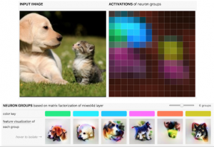
Figure 20: Factorization of the mixed4d layer of GoogLeNet into 6 groups. (Olah et al. 2018)
As always, we can visualize these groups, which continue to exhibit a clear dog-like structure. In fact, these visualizations are clearer than most of the aggregated neurons we observed previously, suggesting matrix factorization simplifies the problem without losing too much information.
Finally, we can apply this factorization across different layers. Similar to saliency maps, we can track how each group in one layer influences the groups in the next layer, all the way to the final classification.
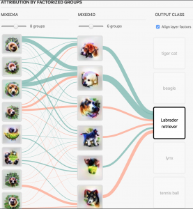
Figure 21: Visualizations and attribution of factorized groups across hidden layers. Blue lines indicate a positive influence on the output class. Red lines indicate a negative influence on the output class. Thicker lines indicate a stronger influence. (Olah et al. 2018)
Here, two hidden layers – thousands of neurons – have been compressed into 14 relatively interpretable images, with clear connections to cats and dogs. Despite being limited to 14 images, through the connecting lines, figure 21 gives a useful “explanation” for its final output.
By simply visualizing and cleverly aggregating neurons, we can peek into the black box. Rather than the separate explainer models of LIME and SHAP, which effectively ignore the hidden layers, the Olah method gives us a sense of how the intermediate representations of the input impact the final output. Because the Olah method lets us observe the inner workings of the model, its explanations are implicitly more trustworthy than those of LIME and SHAP.
The Olah method within the interpretability framework
Still, greater trust in the explanation is traded for poorer explainability. Compared to DeepExplainer, which highlights the importance of individual pixels, the Olah method is harder to digest. For a person inexperienced in machine learning, it would be difficult to apply the Olah method across many images, especially if you wanted to explain why the model chose a labrador retriever instead of a beagle. In such a case, abstract dog visualizations would be uninformative. Moreover, there is a potential observer bias: if a human expects visualizations of dogs and cats, they might miss more abstract but important visualizations, such as the snow in the husky and wolf classification example.
Additionally, the Olah method does not help with simulatability or algorithmic transparency. It disentangles the network enough to provide some sense of decomposability, but perhaps not sufficiently for a non-machine-learning practitioner. Lastly, because this method may be too complex for a layperson, it is not well suited for the taxonomy presented by Doshi-Velez & Kim (2017), which implicitly assumes the humans interpreting the network will not be machine learning experts.
Still, we don’t mean to say this method is bad – far from it. Rather, we want to emphasize that this method is more suited to identifying the role of each subcomponent of a complex model, rather than identifying the features which lead to a decision. For example, in class, we discussed a paper that claims to predict whether someone is a criminal or not from their headshot (Wu & Zhang 2016). The foremost among many criticisms of the paper was that the network was simply a “strain” detector – individuals in the dataset that appeared more strained (because their picture came from a criminal headshot instead of a work photo) were more likely to be criminals. The authors could not effectively respond to this critique, because they were not sure what their model was truly examining when making its decision. The Olah method would allow the authors to do exactly that and would go a long way in showing whether the model had any validity.
Discussion
Having presented several interpretability methods, we want to spend some time discussing them together. However, before considering the individual nuances of LIME, SHAP, and the Olah method, we want to reinforce that the basic nature of interpretability leads to higher-level tradeoffs researchers must consider when building and deploying machine learning models. While some form of interpretability is desired and often necessary, rigidly following requirements for transparency may limit the complexity of models that we are comfortable using. For instance, simple decision trees and linear regression models may be transparent, but they are not powerful enough for many applications for which deep neural networks are currently used.
Then, beyond the tradeoff between powerful models and interpretability, there is also a tradeoff between the various aspects of interpretability among different methods. For example, methods such as LIME and SHAP are compelling tools because they offer simple, decomposable explanations without limiting the power of models. Unfortunately, they may not shed light on the exact workings of the model itself. Further, post-hoc explanations should be taken with a grain of salt. While explanations or visualizations may sit well with the reader, they have the potential to be misleading and may not describe the underlying reason for an algorithmic decision.
On the other hand, the Olah method better describes the inner workings of a model but gives more abstract explanations that might be more useful to machine learning researchers than end-users. As such, we believe that the true benefit of an interpretability framework is being able to formalize these different aspects of interpretability, then pick the most relevant method. The claim “you should use SHAP because it makes your model more interpretable” is largely useless. However, the claim “you should use SHAP because the decomposability it offers is worth the risk of using a post-hoc explanation” makes clear both the benefits and risks of SHAP.
Importantly, the most relevant method can change for different parts of the machine learning pipeline. For debugging a model or showing a model accords with human intuition, the Olah method can provide valuable insight. When that same model is used in production and simple explanations for its decisions are required, SHAP will prove more useful. Other methods may be more useful for finding an interpretable representation of the data, or for cleaning a dataset. With so many options, only with a developed interpretability framework can these different methods be critically compared, allowing researchers to choose the most pertinent one.
Conclusion
In summary, interpretability is desirable in machine learning research because it is how models can be understood and analyzed by humans for real-world applications. Though the concept of “interpretability” is often called upon in literature, interpretability can take many forms – not all of them useful. “Mythos of Model Interpretability” (Lipton 2016) lists the desiderata for which we desire interpretability, and describes the criteria by which the interpretability of models can be analyzed. We use this framework to discuss recent advances in interpretability research – LIME, SHAP, and the Olah method – and the tradeoffs that interpretable models present. Though interpretability research has made large advances, much more remains to be done as machine learning models are deployed and reveal a larger gap between model objectives and real-world costs.
Works Cited
Jay Budzik. Clarifying Why SHAP Shouldn’t Be Used Alone. URL https://www.zest.ai/blog/part-deux-why-not-just-use-shap
Finale Doshi-Velez and Been Kim. 2017. Towards a rigorous science of interpretable machine learning. arXiv preprint arXiv:1702.08608.
Ian Goodfellow. Explaining and Harnessing Adversarial Examples arXiv:1412.6572 [stat.ML]. 2015.
Andrej Karpathy, Fei Fei Li. Deep Visual-Semantic Alignments for Generating Image Descriptions. arXiv:1506.02078 [cs.LG]. 2015.
Trent Kyono, Fiono J Gilbert, Mihaela van der Schaar. Multi-view Multi-task Learning for Improving Autonomous Mammogram Diagnosis. Proceedings of Machine Learning Research 106:1–19, 2019.
Zachary C. Lipton. “The Mythos of Model Interpretability,” https://arxiv.org/pdf/1606.03490.pdf, Jun. 2016.
Scott Lundberg. Interpretable Machine Learning with XGBoost. URL https://towardsdatascience.com/interpretable-machine-learning-with-xgboost-9ec80d148d27.
Scott M Lundberg and Su-In Lee. A unified approach to interpreting model predictions.
In I. Guyon, U. V. Luxburg, S. Bengio, H. Wallach, R. Fergus, S. Vishwanathan, and R. Garnett, editors, Advances in Neural Information Processing Systems 30, pages 4765–4774. Curran Associates, Inc., 2017. URL http://papers.nips.cc/paper/7062-a-unified-approach-to-interpreting-model-predictions.pdf.
Xiaolin Wu and Xi Zhang. Responses to critiques on machine learning of criminality perceptions (addendum of arxiv:1611.04135), 2016. Scott Lundberg, SHAP, (2019), Github repository, https://github.com/slundberg/shap.
Christoph Molnar. “Interpretable machine learning. A Guide for Making Black Box Models Explainable”, 2019. https://christophm.github.io/interpretable-ml-book/.
Chris Olah, Arvind Satyanarayan, Ian Johnson, Shan Carter, Ludwig Schubert, Katherine Ye, and Alexander Mordvintsev. The building blocks of interpretability. Distill, 2018. doi: 10.23915/distill. 00010. https://distill.pub/2018/building-blocks.
Marco T. Ribeiro, Sameer Singh, and Carlos Guestrin. 2016b. “Why should I trust you?”: Explaining the predictions of any classifier. In Knowledge Discovery and Data Mining (KDD).
Cody Marie Wild. One Feature Attribution Method to (Supposedly) Rule Them All: Shapley Values. URL https://towardsdatascience.com/one-feature-attribution-method-to-supposedly-rule-them-all- shapley-values-f3e04534983d