machine learning Research

Analyzing and Improving the Optimization Landscape of Noise-Contrastive Estimation

Authors

Bingbin Liu

Affiliations

Published

November 5, 2021

DOI

Example of an extremely flat loss landscape on Gaussian mean estimation: starting from the noise Q (orange), the NCE loss (blue) flattens out quickly before reaching the ground truth distribution P* (green).

Introduction

Density estimation is the task of estimating the probability density function (pdf) of an unknown distribution. It has been extensively studied in statistics and machine learning, and lies at the core of many real-world applications including language/image generation, anomaly detection, and clinical risk prediction.

A crucial bottleneck to using flexible parametric models, such as large neural networks, is that a density function needs to be normalized, i.e. integrate to one. Thus, if we use $f$ to denote the unnormalized parameterized density, we have to grapple with the normalization constant, also known as the partition function, which is the integral $\int_x f(x)$. Such an integral rarely has an analytical form, and is frequently difficult to even approximate using either Markov Chain Monte Carlo or variational techniques on complex high-dimensional data. Thus, classical approaches to learn parameterized densities from data, such as the Maximum Likelihood Estimator (MLE) are often infeasible.

One way to avoid computing the partition function is to perform Noise Contrastive Estimation (NCE) (Gutmann & Hyvarinen 2010, 2012). The key idea of NCE is to turn the unsupervised learning problem of density estimation into a supervised learning problem of classification, and treat the partition function as an additional parameter of the model that gets updated together with other parameters during the learning process. To estimate a distribution $P_*$ (with pdf $p_*$), NCE makes use of known distribution $Q$ (with pdf $q$) of our choice, often referred to as the “noise” distribution, and trains a parametric discriminant model to distinguish between samples of the target $P_*$ (which we have access to through the training data) and noise $Q$ (which we can generate ourselves). Typically, the proportion of samples from $P_*$ and $Q$ is equal, and the loss of the trained distinguisher is cross entropy. Denoting the distinguisher as $\psi$, we have:

Definition (NCE loss): For data distribution $P_*$, noise $Q$ and estimate $P$, let $\varphi(x) := \log\frac{p}{q}$, then the NCE loss is defined as:
$$L(P)
= -\frac{1}{2}\mathbb{E}_{P_*} \log\frac{1}{1+\exp(-\psi(x))} -\frac{1}{2} \mathbb{E}_{Q} \log\frac{1}{1+\exp(\psi(x))}
$$
or equivalently
$$L(P) = -\frac{1}{2}\mathbb{E}_{P_*} l(x, 1) – \frac{1}{2} \mathbb{E}_{Q} l(x, -1)$$
where $l(x,y) := \frac{1}{1 + \exp(-y\psi(x))}$ is the log sigmoid function.

Given a classifier $\psi$, the implied density estimate for $P$ is $p = q \exp(\psi)$. Why should this yield a good density estimate for $P$? The reason is that the optimal discriminant function which minimizes the population NCE loss is given by $\psi^* = \log p_*/q$, from which we can extract the density $p_*$ since $q$ is known (Menon & Ong 16, Sugiyama et. al. 12). Moreover, NCE is consistent as long as the function class is rich enough to contain the true density ratio function, meaning that given sufficient data, NCE is guaranteed to recover the correct density ratio. Moreover, consistency holds regardless of the choice of $Q$,

In practice though, the choice of $Q$ has a big effect on how well NCE can estimate the underlying density $P_*$. A large distance between $P_*$ and $Q$ has come to be termed a “density chasm” (Rhodes et. al. 20). Prior work has shown that when there is such a density chasm, NCE tends to yield density estimates that are far away from the ground truth under a reasonable computational budget. In other words, the closer $Q$ is to $P_*$, the better — though this is a kind of chicken-and-egg problem, since estimating $P_*$ is what we are trying to do. One intuitive reason why the density chasm results in poor NCE density estimates is that the model does not need to get a good estimate of the density ratio in order to do well in the distinguishing task, especially given a finite number of samples. Figure 1 shows an example of this phenomenon when $P_*$, $Q$ are univariate Gaussians with standard variance and far away means: the NCE loss can be seen to flatten out even when very far away from $P_*$, so that the NCE discriminant function does not need to get close to $P_*$ in order for the loss to be very small.

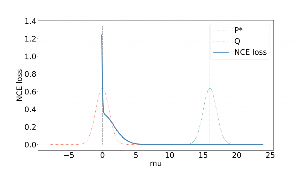Example of density chasm for 1d Gaussian mean estimation: starting from Q (mean 0, gray line), the NCE loss (blue curve) flattens out quickly before reaching the ground truth mean at R = 16 (orange line). The pdfs for Q and P* are shown in red and green.

Multiple prior works have proposed empirical solutions to mitigate the challenges posed by a poorly chosen $Q$ (Rhodes et. al. 20, Gao et. al. 20, Goodfellow et. al. 14). However, these works offered little guidance on when and where they might succeed. The first contribution of this work is to show that the challenges with the density chasm exist even with infinite amounts of data, demonstrating that the problem is not merely a statistical artifact. We then propose a solution, slight modifications to the optimization algorithm and the NCE objective, which provide a simple and provably efficient fix to the problem.

Setup: Exponential family distributions

In this work, we focus on learning distributions from the exponential family. The main reason being that the resulting NCE loss is convex in the exponential family parameters (Uehara et. al. 20): denoting the parameter by $\tau := [\theta, \alpha]$, where $\alpha$ corresponds to the (estimated) log partition function, we have the following result:

Lemma (NCE convexity) For exponential family $p_{\theta, \alpha}(x) = h(x) \exp(\theta^\top \tilde{T}(x) – \alpha)$, the NCE loss is convex in parameter $\tau$.

Flatness of the NCE loss

We first examine the challenges posed to NCE when using a poorly chosen $Q$. The main result of this section is that the difficulty comes from an ill-behaved loss landscape, causing gradient descent and Newton’s method with standard choices of step sizes to fail to find a solution efficiently.

We will prove that such difficulties manifest even in the exceedingly simple special case of Gaussian mean estimation. Namely, we consider the 1d case where $Q = N(0, 1)$ and $P_* = N(R,1)$ for some $R \gg 1$ — the choice of $0$ and $R$ is without loss of generality. Note that since we are providing lower bounds, the simplicity of the setting works in our favor. It is reasonable to expect that the behavior we show can only get worse for more complex or higher dimensional problems.

Let $\tau_*, \tau_q$ denote the parameters of $P_*, Q$, where the log partition function is included as the last coordinate. Let $\tau_t$ denote the parameter of $P$ after $t$ steps of gradient descent. We show that starting from $\tau_0 = \tau_q$, running gradient descent on the NCE objective requires an exponential number of steps to find a good estimate:

Theorem 1 (Lower bound for gradient-based methods)
Let $Q = \mathcal{N}(0, 1)$, $P_* = \mathcal{N}(R, 1)$ with $R \gg 1$. Let $P$ also be 1d Gaussian with variance 1. Then, gradient descent with a step size $\eta = O(R^{-2})$ from an initialization $\tau = \tau_q$ will need an exponential number of steps to reach some $\tau’$ that is $O(1)$ close to $\tau_*$.

Note that the theorem is stated with standard choices of step size $\eta$, that is, $\eta \leq 1 / \sigma_{M}$ where $\sigma_{M}$ is smoothness of the loss function. It is possible that clever choices of $\eta$, such as an adaptive schedule, can avoid the exponential lower bound. (Stay tuned!)

The proof idea is to show that there is an annulus surrounding $\tau_*$, of width $\Theta(R)$, but where the gradient norms are roughly $O(\exp(-R^2/8))$. Thus, even with constant step sizes, it would take gradient descent an exponential number of steps to cross the annulus. Moreover, the optimization path has to cross this region since the starting point $\tau_q$ and the target $\tau_*$ lie on different sides of the annulus (see Figure 2 for an illustration), hence the total number of optimization steps has to be exponential.

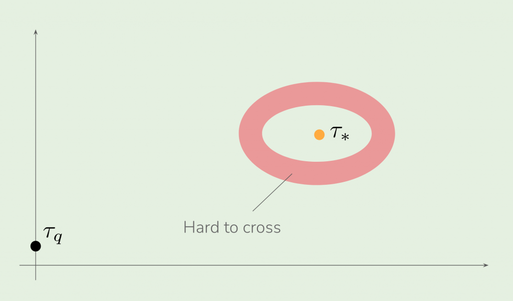Figure 2: The initial $\tau_q$ and target parameter $\tau_*$ lie on different sides of the red annulus, hence the optimization path has to pass through the annulus. However, the gradient norm is exponentially small in the annulus, which means it takes an exponential number of steps to cross the annulus, hence the entire optimization process requires an exponential number of steps.

The lower bound in Theorem 1 arises due to drastically changing norms of the gradients. A natural remedy for this is to use methods that can precondition the gradient, which motivates the use of second order methods. Unfortunately, we show using a similar argument as the gradient descent analysis that standard second-order approaches are again of no help, and the number of steps required to converge remains exponential:

Theorem 2 (Lower bound for Newton’s method) Let $P_*, Q, P$ satisfy the same conditions as in Theorem 1. Let $\sigma_{\rho}, \sigma_M$ denote the global strong convexity and smoothness constants.
Then, running the Newton’s method with a step size $\eta = O(\frac{\sigma_{\rho}}{\sigma_{M}})$ from an initialization $\tau = \tau_q$ needs an exponential number of steps to reach some $\tau’$ that is $O(1)$ close to $\tau_*$.

Here the choice of step size $\eta$ again follows the standard choice, that is, it should be upper bounded by the ratio between the global strong convexity and smoothness constants. Note also that the analyses are on the population level, implying that the hardness comes from the landscape itself regardless of the statistical estimators used.

Solution: Normalized Gradient Descent (NGD) with the eNCE objective

We have seen that due to an ill-behaved landscape, optimizing the NCE objective with standard gradient descent or Newton’s method will fail to reach a good parameter estimate efficiently.

In this section, we propose a solution that guarantees a provably polynomial rate. Our approach combines two key ideas: the well-studied Normalized Gradient Descent (NGD) and a new loss function we call the eNCE.

Recall that a NGD step is similar to a standard gradient descent step except that the gradient is now normalized:
$$\tau_{t+1} = \tau_t – \eta \frac{\nabla L(\tau_t)}{|\nabla L(\tau_t)|_2}.$$

Returning to the 1d Gaussian mean estimation task as an example, the effectiveness of NGD comes from the crucial observation that even though the magnitude for the loss and its gradients can be exponentially small, they are exponentially small to the same order (i.e., they share the same exponential factor). This exponential factor cancels out during normalization, hence eliminating the convergence difficulties faced by standard GD.

For exponential families in general, we can show that when the singular values of the Hessian around the target parameter $\tau_*$ change moderately, NGD can find a parameter with target error $\delta$ in $O(1/\delta^2)$ steps:

Theorem 3 (Guarantee on NGD, informal) Let $P_*, Q$ be exponential family distributions with parameters $\tau_, \tau_q$. Initialize the parameter estimate at $\tau_0$. Assuming the log partition function is $\beta_Z$ Lipschitz, and that the Hessian $\mathbf{H}$ are such that $\frac{\sigma_{\max}(\mathbf{H}(\tau))}{\sigma_{\max}(\mathbf{H}(\tau_*))} \leq \beta_u$, $\frac{\sigma_{\min}(\mathbf{H}(\tau))}{\sigma_{\min}(\mathbf{H}(\tau_*)} \geq \beta_l$, $\forall \tau$ where $ \|\tau – \tau_*\|_2 \leq \frac{1}{\beta_Z}$, then for any $\delta \leq \frac{1}{\beta_Z}$, NGD finds an estimate $\tau$ such that $\|\tau – \tau_*\|_2 \leq \delta$ within $\frac{\beta_u \kappa_*}{\beta_l} \frac{\|\tau_0 – \tau_*\|_2^2}{\delta^2}$ steps, where $\kappa_*$ is the condition number of the NCE Hessian at the optimum.

Remarks: Theorem 3 subsumes Gaussian mean estimation as a special case, hence NGD provides a solution that avoids the exponential lower bound in Theorem 1.

One the positive side, Theorem 3 says that under some assumptions, NGD gives a rate polynomial in the parameter distance and condition number $\kappa_*$. The remaining question though is that it is not yet clear how $\kappa_*$ behaves. For example, if $\kappa_*$ itself were to grow exponentially in the parameter distance between $\tau_*$ and $\tau_q$, then the rate from NGD would still be exponential and the problem would remain.

Fortunately, we will show that for a slight modification to the NCE loss, which we call the eNCE objective, $\kappa_*$ indeed grows polynomially in the parameter distance and class-related constants. This means though eNCE may still suffer from the flatness problem when using gradient descent, eNCE and NGD together provide a solution that guarantees a polynomial convergence rate.

Formally, the eNCE loss is defined as:

Definition (eNCE loss) Let $\varphi(x) := \log\sqrt{\frac{p(x)}{q(x)}}$. The NCE loss of $P_\tau$ w.r.t. data distribution $P_*$ and noise $Q$ is:
$$
L_{\text{exp}}(P_{\tau})
= \frac{1}{2} \mathbb{E}_{x\sim P_*} [l\left(x, 1\right)] + \frac{1}{2}\mathbb{E}_{x\sim Q} [l\left(x, -1\right)] = \frac{1}{2}\int_x p_*\sqrt{\frac{q(x)}{p(x)}} + \frac{1}{2}\int_x q\sqrt{\frac{p(x)}{q(x)}}
$$
where $l(x, y) = \exp(-y \varphi(x))$ is the exponential loss and $y \in {\pm 1}$.

Just as with the original NCE loss, the eNCE loss is constructed in two steps. Given a density estimate $P$, we use it to construct a classifier estimate $\varphi = \log \sqrt{p/q}$; or alternatively, we could start with a classifier estimate $\varphi$, which represents the density estimate $p = q \exp(2\varphi )$. The eNCE loss is then simply the exponential classification loss of using $\varphi(x)$ to distinguish between samples of $P_*$ and samples of $Q$. The use of the exponential loss, rather than the cross-entropy loss in the original NCE, is why we term this loss the eNCE loss. Note that we also have a different parameterization of the discriminant $\varphi$ in terms of the densities $p,q$. It’s also easy to check that the minimizing $\varphi$ learns the log density ratio, i.e. $\varphi(x) = \frac{1}{2}\log\frac{p_*}{q}$, hence eNCE can recover $p_*$ given $q$ as NCE does.

The main advantage of using the eNCE loss is that the condition number $\kappa_*$ is now provably polynomial in certain class-dependent constants. The intuition of the proof is that the Hessian of the eNCE objective has a nice algebraic form, hence the choice of $P_*, Q$ doesn’t affect the condition number except via a class-dependent constant. As a result, we show that:

Theorem (eNCE convergence with NGD, informal) Let $P_*, Q$ be exponential family distributions with parameters $\tau_*, \tau_q$. Assuming the log partition function is $\beta_Z$-Lipschitz, then for any given $\delta \leq \frac{1}{\beta_Z}$ and parameter initialization $\tau_0$, performing NGD on the eNCE objective finds an estimate $\tau$ such that $|\tau – \tau_*|_2 \leq \delta$ within $T = O\left(\frac{|\tau_0 – \tau_*|^2}{\delta^2}\right)$ steps, where the $O(\cdot)$ notation hides class-dependent constants.

This means combining NGD with the eNCE objective guarantees a polynomial convergence rate.

Experiments

The goal of this work is to understand and improve the “density chasm” problem, which says that NCE can suffer from a poor performance in practice when the noise distribution $Q$ is far from $P$. In the previous sections, we have identified one source of the problem to be an ill-behaved landscape, and proposed a combination of NGD and eNCE as a fix for a provably polynomial guarantee. Our analysis suggests that in theory, NGD should be more robust to the choice of noise distribution Q. We would now like to verify these results empirically on Gaussian data and MNIST.

For Gaussian, we experiment with 1d and 16d data, and plot the parameter distance against the number of update steps in Figure 3. We can see that under a fixed computation budget, 1) normalized gradient descent (NGD) indeed outperforms gradient descent (GD), and that 2) the proposed eNCE loss performs comparatively, and in many cases, even decays faster compared to NCE while additionally enjoys provable polynomial convergence guarantees.

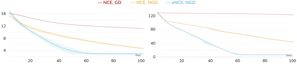Figure 3: Results for estimating 1d (left) and 16d (right) Gaussian, plotting the best parameter distance so far (y-axis) against the number of optimization iterations (x-axis). In both cases, when using NCE, normalized gradient descent (“NCE, NGD”, yellow curve) significantly outperforms gradient descent (“NCE, GD”, red curve). When using NGD, the proposed eNCE (“eNCE , NGD”, blue curve) also decays faster than the original NCE loss. The results are averaged over 5 runs, with the shaded area showing the standard deviation.

For MNIST, we can no longer compare parameter distance since the ground truth parameter $\tau_*$ is unknown. We instead compare the loss curves directly, and Figure 4 shows that NGD outperforms GD for both the NCE and eNCE loss.

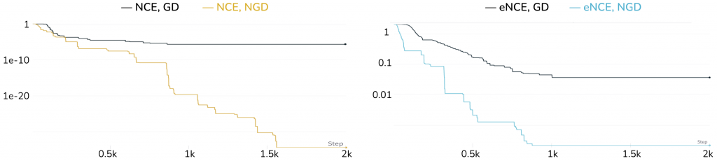Figure 4: Results on MNIST, plotting the loss values (y-axis, log scale) against the number of updates (x-axis). The left plot shows NCE optimized by GD (black) and NGD (yellow), and the right shows eNCE optimized by GD (black) and NGD (blue). NGD outperforms GD in both cases.

Conclusion

In this blog post we identified an ill-behaved loss landscape as a key reason for the “density chasm” difficulties when optimizing the NCE objective with a far away noise distribution. A consequence of this is that these “density chasm” issues are not mere statistical artifacts: they arise even given access to infinite data. We saw that even on the simple task of Gaussian mean estimation, and even assuming access to the population gradients, gradient descent and Newton’s method with standard step size choices still require an exponential number of steps to reach a good solution.

To address these issues caused by a flat landscape, we propose a combination of changing the loss and the optimization algorithm. The loss we introduce, eNCE, can be efficiently optimized using normalized gradient descent. There is lots of room for future exploration, including formalizing the finite-sample behavior of NGD and eNCE.

Refereneces

Ruiqi Gao, Erik Nijkamp, Diederik P Kingma, Zhen Xu, Andrew M Dai, and Ying Nian Wu. Flow contrastive estimation of energy-based models. In CVPR 2020.
Ian J Goodfellow, Jean Pouget-Abadie, Mehdi Mirza, Bing Xu, David Warde-Farley, Sherjil Ozair, Aaron Courville, and Yoshua Bengio. Generative adversarial networks. In NeurIPS 2014.
Michael Gutmann and Aapo Hyvärinen. Noise-contrastive estimation: A new estimation principle for unnormalized statistical models. In AISTATS 2010.
Michael U Gutmann and Aapo Hyvärinen. Noise-contrastive estimation of unnormalized statistical models, with applications to natural image statistics. Journal of Machine Learning Research, 13(2), 2012.
Aditya Menon and Cheng Soon Ong. Linking losses for density ratio and class-probability estimation. In ICML 2016.
Benjamin Rhodes, Kai Xu, and Michael U Gutmann. Telescoping density-ratio estimation. NeurIPS 2020.
Masashi Sugiyama, Taiji Suzuki, and Takafumi Kanamori. Density Ratio Estimation in Machine Learning. Cambridge University Press, 1st edition, 2012.
Masatoshi Uehara, Takafumi Kanamori, Takashi Takenouchi, and Takeru Matsuda. A unified statistically efficient estimation framework for unnormalized models. In AISTATS 2020.

380 6952
Read More

Machine Learning Blog | ML@CMU | Carnegie Mellon University

Statistics:

Categories: