Based on: Potosnak, W., Wolff, M., Cao, M., Ma, R., Konstantinova, T., Efimov, D., Mahoney, M.W., Oreshkin, B., & Olivares, K.G. "Forking-Sequences: Statistically and Computationally Efficient Multi-Horizon Forecasting with Reduced Volatility." Transactions on Machine Learning Research, 2026.

(Disclaimer: Code implementation not used in the paper; not affiliated with Amazon — provided as a reference for forking-sequences and forecast ensembling)
TL;DR
-
One architectural swap, no new parameters. Instead of encoding one forecast window at a time in the window-sampling training paradigm, forking-sequences encodes and decodes the entire series across all forecast creation dates in a single forward pass.
-
Encoder-Agnostic. Validated across six encoder types — MLP, RNN, LSTM, CNN, Transformer, and State Space.
-
Better gradients, faster training. Loss is pooled across every forecast creation date, cutting gradient variance at a linear rate and fixing vanishing gradients in RNNs/LSTMs — sCRPS improved up to 49.3% for LSTM encoders.
-
Order-of-magnitude cheaper inference. Reusing encoder outputs across T forecast dates cuts cross-validation complexity by a factor of T for every encoder type — e.g. for LSTMs, RNNs, and CNNs, O(T²) drops to O(T).
Multi-horizon forecasting has become the default approach across energy, finance, supply chain, and healthcare applications, because it gives planners visibility into entire future trajectories rather than single-point outcomes, supporting short-, medium-, and long-term planning alike. But how a model is trained has a surprisingly large effect on both statistical and computational efficiency as well as accuracy, and one of the most powerful architectural choices for this is also one of the most underexplored: forking-sequences.
Forking-sequences has informed the design of MQForecaster neural networks for industrial applications, with notable examples including MQCNN [1], MQT [2], and SPADE [3]. Yet, until now, it hadn't been formally defined, theoretically justified, or systematically benchmarked. This post walks through what forking-sequences is, why it's a statistically and computationally more efficient training paradigm, and how it impacts forecast accuracy across different encoder types. Part II covers the companion benefit: reduced forecast volatility through ensembling.
Window-Sampling vs. Forking-Sequences
Most neural forecasting models use a standard architectural design known as window-sampling. In this setup, the model encodes a fixed-length window of history and decodes a single multi-horizon forecast from it. The window-sampling approach segments the series into windows of size L; and windows are treated independently across each forecast creation date (FCD), or the point in time from which a forecast is issued. The Encoder outputs a hidden state for each position in the forecast horizon; we use [h] = [1, ..., H] to index the embedding corresponding to each horizon step h:
\[
\mathbf{h}_{t,[h]} = \mathrm{Encoder}\left(\mathbf{Y}_{[t]}\right) \qquad \text{and} \qquad %\
\hat{\mathbf{Y}}_{t,[h]} = \mathrm{Decoder}\left(\mathbf{h}_{t,[h]}\right) .
\]
Window-sampling is portrayed in Fig. 1.
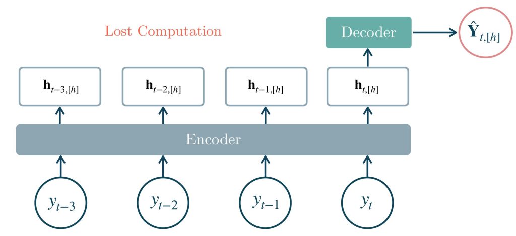 Fig. 1: Window-sampling
Forking-sequences takes a different approach: it jointly encodes and decodes the entire time series across all FCDs in a single forward pass, producing a full grid of multi-horizon forecasts at once. Instead of a single hidden state per window, the encoder outputs a hidden representation for every FCD, and a shared decoder turns each of those into its own multi-horizon forecast:
\[
\mathbf{h}_{[t][h]} = \mathrm{Encoder}\left(\mathbf{Y}_{[t]}\right) \qquad \text{and} \qquad %\\
\hat{\mathbf{Y}}_{[t][h]} = \mathrm{Decoders}\left(\mathbf{h}_{[t][h]}\right).
\]
Forking-sequences is portrayed in Fig. 2.
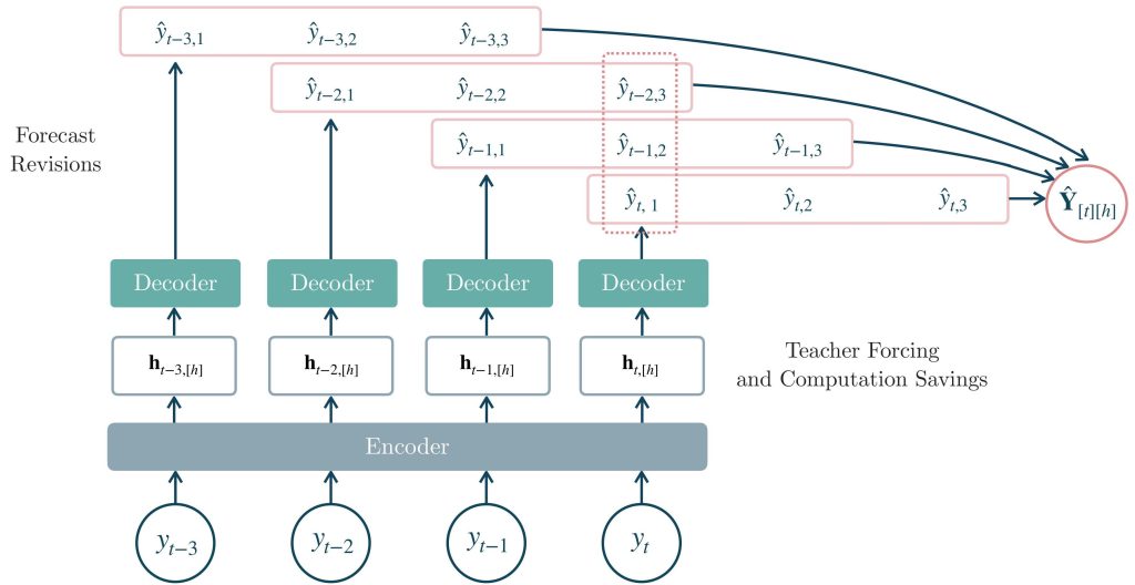
Fig. 2: Forking-sequences
Ideas similar to forking-sequences have been present in the forecasting literature for decades, despite not inspiring neural network architectural design or training. Most notably, [4] introduced time-series cross-validation as a model selection technique that accounts for temporal dynamics and data dependencies, addressing the limitations of classical cross-validation; this approach assumes independent FCD observations.
Forking-sequences also shares conceptual similarities with the teacher-forcing technique, most notably through the next-token prediction objective [5], which is an autoregressive learning strategy which trains models to predict the next token given previous ones. However, a key difference between the standard teacher-forcing technique used in NLP autoregressive models and the forking-sequences approach used in neural forecasting is the implicit target replication that arises in multi-horizon forecasts. Whereas NLP models are typically trained to predict only the next token, forecasting models must predict longer future trajectories, generating multiple future steps for each FCD. This difference aside, forking-sequences does the analogous thing for time series: it converts one series into a full set of overlapping multi-horizon training targets, multiplying the supervision signal extracted from each series at negligible extra cost.
Benefit 1: Statistical Efficiency (Better Gradients)
During training, the gradients are computed with respect to the model parameters for SGD updates to minimize the loss. We use Quantile Loss (QL) in our experiments. The gradient is computed on a B-length minibatch. With a window-sampling architecture, multi-horizon losses are gathered in a batch B for individual FCDs:
\[
\nabla \mathcal{L} =
\frac{1}{B \times H}
\sum^{B}_{b=1} \sum^{H}_{h=1}
\nabla \mathrm{QL} \left(y_{b,h},\; \hat{y}_{b,h}). \right .
\]
With forking-sequences, the gradient is computed from losses gathered across all T FCDs in the series simultaneously for B-length minibatch of individual time series:
\[
\nabla \mathcal{L}_{T} =
\frac{1}{B \times T \times H}
\sum^{B}_{b=1} \sum^{T}_{t=1} \sum^{H}_{h=1}
\nabla \mathrm{QL} \left(y_{b,t,h},\; \hat{y}_{b,t,h} \right) .
\]
The paper proves a key theoretical result:
Theorem 1 (Forking-Sequences SNR Gains under M-Dependence).
If the T gradient samples are M-dependent, the forking-sequences gradient estimator's variance decreases linearly (O(1/T)), and its signal-to-noise ratio (SNR) grows linearly (O(T)).
In plain terms: forking-sequences pools gradient information across many FCDs within a single series. Because these samples are only locally correlated (temporally close FCDs are dependent, but that dependence vanishes beyond a bounded lag), averaging over more of them drives the gradient estimator's variance down at a linear rate, O(1/T) in the number of FCDs, the same mechanism behind the classical weak law of large numbers. This has a twofold effect in improved statistical efficiency:
- Improved gradient Signal-to-Noise (SNR), which translates to smoother optimization trajectories and faster convergence, as shown in Fig. 3.
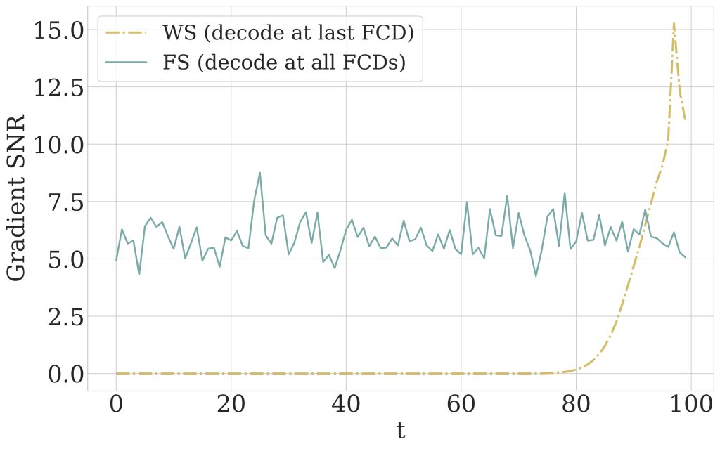
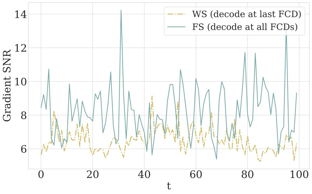
- Mitigated vanishing gradients, particularly for recurrent architectures like RNNs and LSTMs as shown in Fig. 4. Because forking-sequences decodes losses at every FCD rather than only the last one, gradients are preserved for early time steps instead of decaying exponentially through backpropagation-through-time.
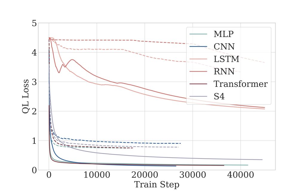 (a) Train set
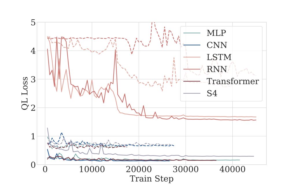 (b) Validation set
Fig. 3: MQForecaster model optimization convergence on the M4 hourly data, using either forking-sequences (solid) or window-sampling (dashed) techniques. Quantile loss on the (a) train set and (b) validation set as a function of train steps are consistently lower for forking-sequences models. Across architectures forking-sequences show validation quantile loss improvements.
 (a) LSTM gradient SNR
 (b) Transformer gradient SNR
Fig. 4: Forking-sequences yields higher gradient signal-to-noise ratio (SNR) for LSTMs, indicating more stable training signals. Transformer gradient SNR remains relatively stable for both forking-sequences and window-sampling, as Transformers do not suffer from vanishing gradients.
Benefit 2: Computational Efficiency
Beyond training, forking-sequences also makes inference substantially cheaper, particularly for cross-validation style inference, where a model needs to generate forecasts at many rolling FCDs.
Window-sampling recomputes the encoder from scratch at every FCD. Since consecutive rolling windows overlap heavily, most of that recomputation is redundant, the encoder is reprocessing input it has effectively already seen, just to throw the result away and start over at the next FCD. Forking-sequences avoids this entirely: it encodes the full series once, propagating hidden states forward across FCDs instead of recomputing them from scratch each time.
Fig. 5: Empirical validation of computational complexity through wall-clock measurements across different inference methods. T represents the time series length, and L denotes the window size in restricted window-sampling.
The headline "factor of T" speedup is measured against window-sampling (full; unrestricted history), where each FCD's encoder reprocesses the entire history seen so far. For LSTMs, CNNs, and RNNs, this drops complexity from O(T²) to O(T). For Transformers, unrestricted self-attention costs O(T³) (each of T FCDs redoing an O(T²) attention pass), while forking-sequences does it once at O(T²), the same T-fold gain as shown in Table 1.
Table 1: Theoretical encoder complexity for forking-sequences (FS) vs. restricted window-sampling (WS restr.) vs. full window-sampling (WS full). T = number of FCDs, L = window size.
|
MLP |
CNN |
RNN |
Attention |
S4 |
| FS |
O(T) |
O(T) |
O(T) |
O(T2) |
O(T log T) |
| WS restr. |
O(TL) |
O(TL) |
O(TL) |
O(TL2) |
O(TL log L) |
| WS full |
O(T2) |
O(T2) |
O(T2) |
O(T3) |
O(T2 log T) |
In practice, though, Transformers often use a fixed, restricted window (a bounded lookback of length L) rather than unbounded history, due to the quadratic complexity of full attention. Against this baseline, forking-sequences' O(T²) only outperforms restricted window-sampling's O(T·L²) when T < L². To retain both the statistical and computational benefits of forking-sequences in this regime, FCDs can be sampled into segments where T ≤ L², rather than applied across the full series length.
Empirical Results: Accuracy Gains Across the M-Series Benchmark
To assess training paradigm impact on forecast accuracy, we trained MQForecaster models varying only the encoder (MLP, RNN, LSTM, CNN, Transformer, State Space/S4) with forking-sequences vs. window-sampling, and evaluated on 16 datasets spanning the M1, M3, M4, and Tourism competitions, using scaled Continuous Ranked Probability Score (sCRPS) and Mean Absolute Error (MAE) as accuracy metrics.
 (a) sCRPS
 (b) MAE
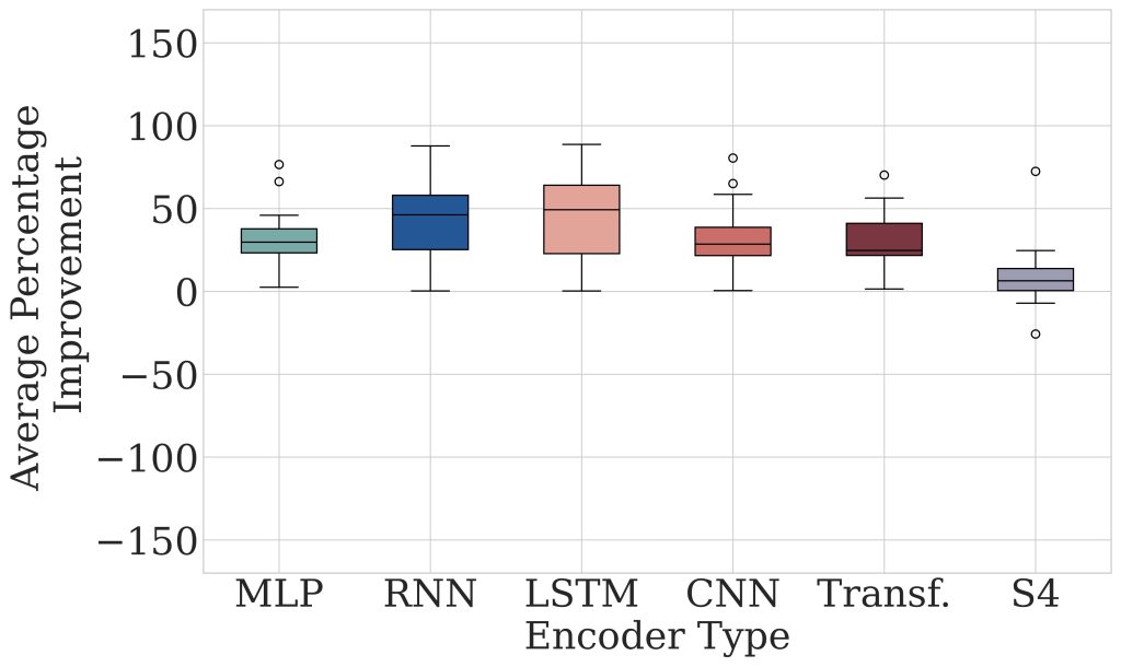
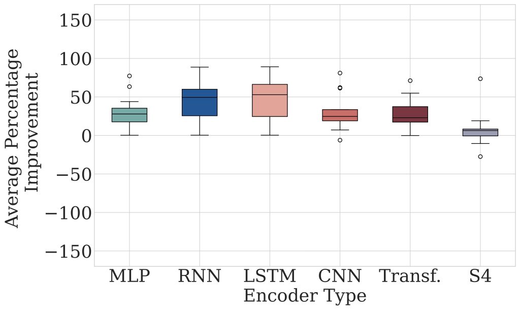
Fig. 6: Distribution of percentage improvement in (a) sCRPS and (b) MAE metrics across datasets for different encoder types trained with forking-sequences compared with window-sampling. Each dataset's metric is averaged over 5 random seed runs. Percentage improvement greater than zero indicates forking-sequences achieves lower forecast error.
While all encoder variants with forking-sequences show improved sCRPS, the magnitude of improvement notably varies across encoder architectures and individual datasets as visualized in Fig. 6, which shows the distribution of percentage improvement in sCRPS and MAE metrics across datasets for different encoder types trained with forking-sequences compared with window-sampling. For LSTM encoder models, training with forking-sequences reduced sCRPS by 49.3%, on average across datasets, compared to the window-sampling scheme. Consistent median gains across datasets are observed for RNN (46.2%), and CNN (28.6%) encoders, while the Transformer (24.7%) and StateSpace (6.4%) encoders showed smaller improvement.
We hypothesize these performance differences stem from how well each encoder architecture propagates gradients on its own. Transformers use self-attention, which lets every timestep attend directly to every other timestep, so gradients don't have to pass through a long sequential chain the way they do in RNN/LSTM backpropagation-through-time. This means Transformers largely avoid the vanishing-gradient problem to begin with, so forking-sequences' statistical benefit of preserving gradients for early timesteps has less room to help. LSTMs, by contrast, do suffer from vanishing gradients under standard backpropagation-through-time, which forking-sequences directly mitigates. We confirm this empirically in Fig. 4, which shows a higher gradient SNR for LSTM encoders under forking-sequences, while Transformer SNR stays comparable between the two schemes.
🔑 Takeaways
1
Forking-sequences is not a new loss function or a new architecture, it's a training and inference paradigm that's encoder-agnostic and can be retrofitted onto CNNs, RNNs, LSTMs, Transformers, and state-space models alike.
2
It improves gradient quality (lower variance, higher SNR) in a way that's theoretically grounded and empirically validated, especially benefiting architectures prone to vanishing gradients.
3
It cuts inference-time computational complexity by an order of magnitude for cross-validation style workflows.
4
All encoder variants with forking-sequences show median improved sCRPS across datasets. The magnitude of improvement notably varies across encoder architecture, with the biggest gains for RNN- and LSTM-based encoders.
Up next: In Part II, we cover another aspect of forking-sequences: how the same architecture naturally supports efficient forecast ensembling across FCDs, why that matters for reducing forecast volatility, and considerations for reducing forecast volatility without sacrificing accuracy.
References:
[1] Ruofeng Wen, Kari Torkkola, Balakrishnan Narayanaswamy, and Dhruv Madeka. A Multi-horizon Quantile Recurrent Forecaster. In 31st Conference on Neural Information Processing Systems NIPS 2017, Time Series Workshop, 2017.
[2] Carson Eisenach, Yagna Patel, and Dhruv Madeka. MQTransformer: Multi-Horizon Forecasts with Context Dependent and Feedback-Aware Attention. In Maria Florina Balcan and Marina Meila, editors, Submitted to Proceedings of the 38th International Conference on Machine Learning. PMLR. Working Paper version available at arXiv:2009.14799, 8 2021.
[3] Malcolm Wolff, Kin G. Olivares, Boris Oreshkin, Sunny Ruan, Sitan Yang, Abhinav Katoch, Shankar Ramasubramanian, Youxin Zhang, Michael W. Mahoney, Dmitry Efimov, and Vincent Quenneville-Bélair. ♠ SPADE ♠: Split Peak Attention DEcomposition. In Thirty-Eighth Annual Conference on Neural Information Processing Systems NeurIPS 2024, volume Time Series in the Age of Large Models Workshop, Vancouver, Canada, 2024. NeurIPS 2024.
[4] Jeffrey D. Hart. Automated kernel smoothing of dependent data by using time series cross- validation. Journal of the Royal Statistical Society. Series B (Methodological), 56(3):529–542, 1994.
[5] Yoshua Bengio, Réjean Ducharme, Pascal Vincent, and Christian Jauvin. A neural probabilistic language model. Journal of Machine Learning Research, 3:1137–1155, 2003.
