Based on: Potosnak, W., Wolff, M., Cao, M., Ma, R., Konstantinova, T., Efimov, D., Mahoney, M.W., Oreshkin, B., & Olivares, K.G. "Forking-Sequences: Statistically and Computationally Efficient Multi-Horizon Forecasting with Reduced Volatility." Transactions on Machine Learning Research, 2026.

(Disclaimer: Code implementation not used in the paper; not affiliated with Amazon — provided as a reference for forking-sequences and forecast ensembling)
TL;DR
-
Ensembling, nearly for free. Forking-sequences already produces overlapping forecasts for every target date across FCDs in a single forward pass, so ensembling them at inference adds no extra encoder computation compared with window-sampling.
-
Two new forecast volatility metrics. scaled Forecast Percentage Change (sFPC) measures raw revision size in real time (no ground truth needed); Excess Volatility (EV) goes further, rewarding accuracy-improving revisions and only penalizing the ones that move forecasts away from the truth or overshoot it.
-
Reduced volatility without sacrificing accuracy. Exponential-smoothing forecast ensembling (α = 0.9) reduces sEV by 10–13% across all encoder types, with less than 0.1% accuracy degradation.
-
Works zero-shot on models pretrained with window-sampling. Forecast ensembling applied to pretrained Time Series Foundation Models (TSFMs) — Chronos-2, Toto 2.0, TimesFM, PatchTST, N-BEATS — cuts volatility by ~10% with negligible accuracy cost (less than 0.1%).
In Part I, we introduced forking-sequences, a neural network architectural design that jointly encodes and decodes a time series across all forecast creation dates (FCDs) in a single forward pass. We showed why it's a statistically and computationally more efficient training paradigm than window-sampling. In Part II, we turn to a different but equally important problem: forecast volatility.
Why Forecast Volatility Matters
Accuracy is usually the headline metric for a forecasting model, but it isn't the only thing that matters in production. As a multi-horizon forecasting system operates over time, it generates multiple overlapping forecasts for the same future target date — one from each new FCD as more data becomes available. This sequence of updates is a forecast revision, and how consistent (or erratic) those revisions are is what we define as forecast volatility.
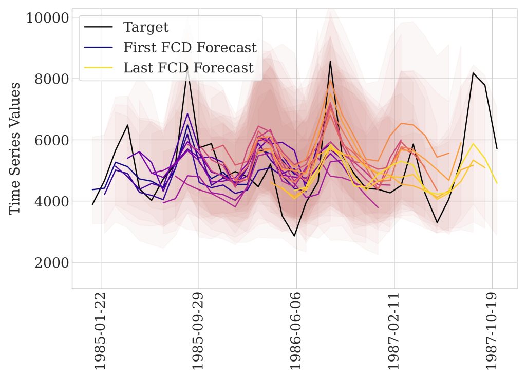 (a) Without forecast inference ensembling
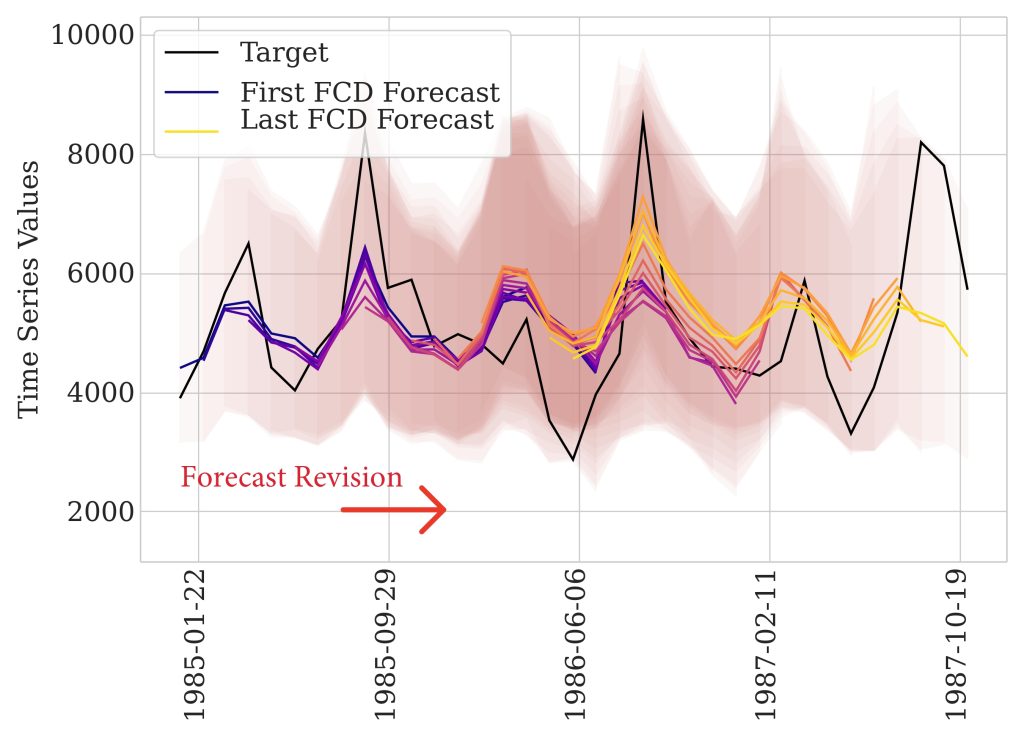 (b) With forecast inference ensembling
Fig. 1: Forecasts (a) without and (b) with forecast ensembling applied. Forecast ensembling reduces volatility across FCDs, resulting in more stable and consistent forecast distributions. Red arrows indicate the direction of forecast revisions. Lines show P50 (median) forecasts across different FCDs. By reusing encoder computations, forking-sequences enables computationally efficient forecast ensembling with negligible additional cost.
Consider an electrical grid operator using load forecasts to plan power supply. If a forecast revises from 45 GW to 65 GW ahead of a heat wave, that's a useful revision; it tells operators to activate reserve plants. But if forecasts jump around erratically between FCDs without new information justifying the change, that undermines trust and complicates planning. The goal isn't to eliminate revisions, it's to distinguish benign, informative revisions from excessive, erratic ones.
This raises two questions we tackle directly in the paper:
?
How do we measure forecast volatility in a way that separates useful revisions from harmful ones?
?
Are there architectural designs that reduce volatility without hurting accuracy?
Forking-Sequences as a Natural Forecast Ensembling Mechanism
Because forking-sequences generates forecasts for every FCD in a single forward pass, it naturally produces multiple overlapping predictions for the same target date. Recall the forecast revision relationship: the prediction for a given target made at FCD t+1 is a revision of the prediction made at FCD t for the same date. Forecast revisions with the forking-sequences paradigm are shown in Fig. 2.
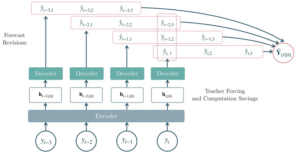 Fig. 2: Forking-sequences
This overlapping grid structure means forking-sequences models can be ensembled for free (or nearly so) at inference time in terms of saving encoder computation compared with window-sampling, which requires multiple independent model forward passes. Given forecasts outputs via forking-sequences, we just average (or otherwise combine) the different FCD-level predictions for the same target date portrayed as the diagonal band in Fig. 3a:
\[
\begin{equation}
\widetilde{\mathbf{Y}}_{t,h} = \frac{1}{H}\sum_{k=0}^{H} \widehat{\mathbf{Y}}_{t-k, h+k} \qquad \text{for } t\geq H.
\label{eq:forking_sequences_ensemble}
\end{equation}
\]
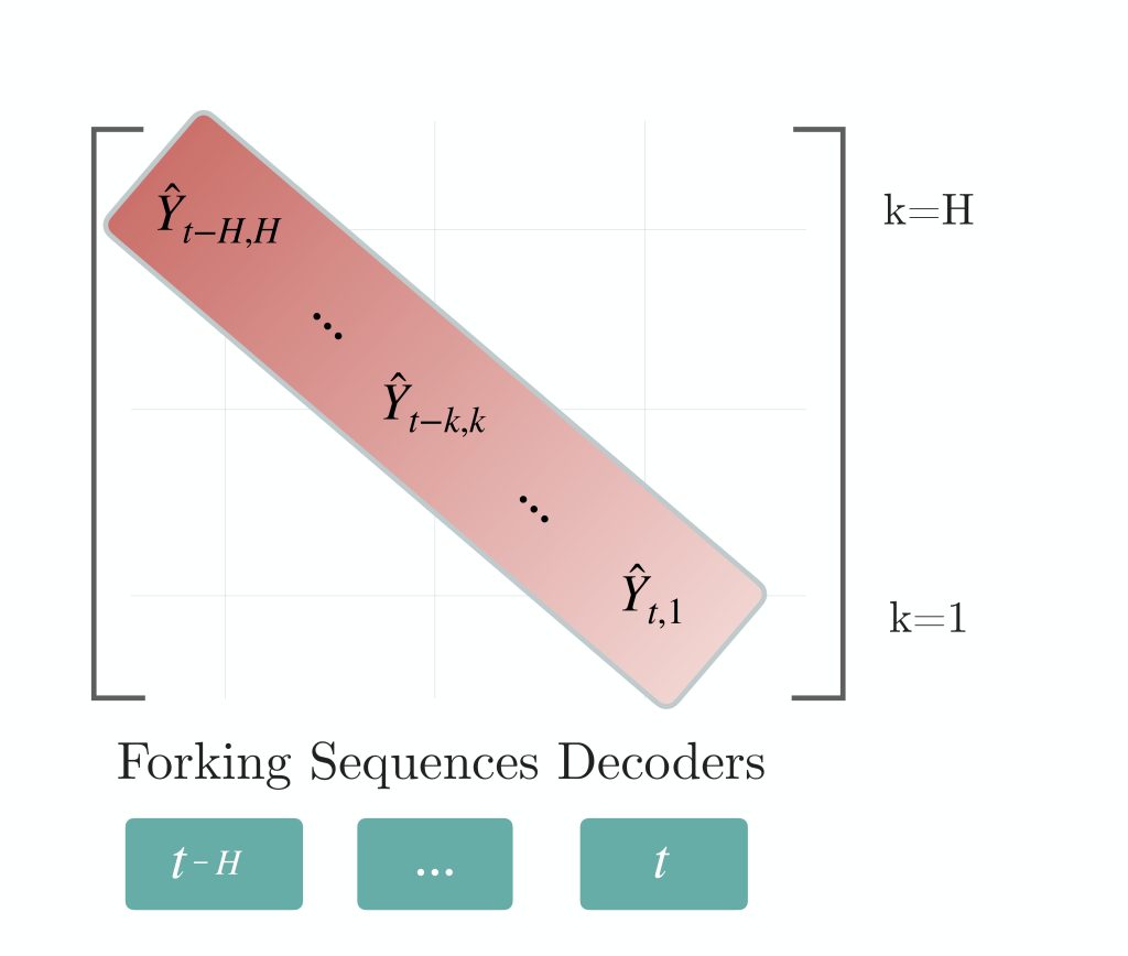 (a) Forking-sequences forecast ensemble
 (b) Forecast volatility reduction
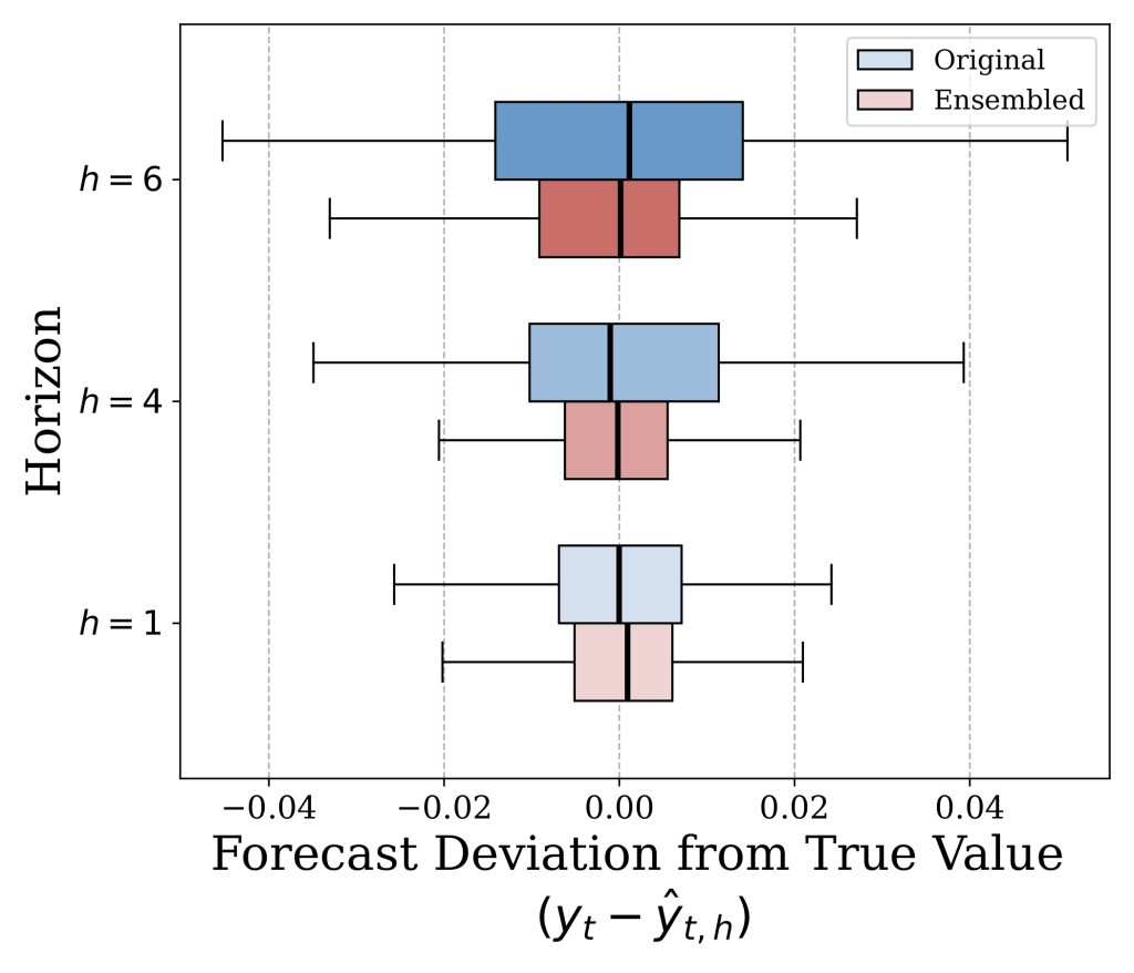
Fig. 3: We adapt forking-sequences during inference to ensemble multiple forecasts of the same future date by computing a function (ex., moving average) across predictions generated from previous FCDs. b) Forking-sequences ensembling reduces forecast volatility, reducing the estimators variance with a linear convergence rate analogous to the weak law of large numbers.
Although it is tempting to expect a variance-reduction behavior similar to the results of Theorem 1, it is important to recognize that forecast variance naturally increases the further a forecast is from its corresponding observation. As a result, there is an inherent limit to how much ensembling can reduce volatility: older forecast revisions carry substantially higher uncertainty, whereas more recent revisions are both more accurate and less variable. This makes it desirable for an ensemble to place greater weight on newer forecasts rather than treating all revisions equally.
New Forecast Volatility Metrics
We introduce scaled Forecast percentage Change (sFPC) to measure the relative change in predicted quantiles across consecutive forecast creation dates, providing a quantitative view of temporal volatility or forecast revision rates. Inspired by the sMAPE metric, sFPC uses a symmetric denominator, based on both current and previous forecasts, to mitigate issues of numerical instability [1]. This design ensures robustness when dealing with small predicted values and avoids the division-by-zero problems common in traditional percentage-based metrics.
\[
\mathrm{sFPC}^{(q)}\left(\hat{\mathbf{y}}^{(q)}_{[b][t][h]}\right)
= \frac{200}{B \times T \times H} \sum_{b,t,h} \frac{|\hat{y}^{(q)}_{b,t+1,h}-\hat{y}^{(q)}_{b,t,h+1}|}{|\hat{y}^{(q)}_{b,t+1,h}| + |\hat{y}^{(q)}_{b,t,h+1}|} .
\]
Computing sFPC between consecutive forecasts treats all revisions as equally undesirable, even ones that clearly improve accuracy. To address this, we also introduce scaled Excess Volatility (sEV), a metric for probabilistic forecasts that only penalizes revisions that move a forecast away from the truth, or that overshoot it. sEV is designed to reward accuracy-improving forecast revisions while distinguishing them from harmful volatility. sEV is defined as:
\[
\mathrm{sEV}\left(\mathbf{y}_{[b][t][h]}, \hat{\mathbf{y}}_{[b][t][h]}\right) = \frac{\sum_{b,t,h} \mathrm{EV}(y_{b,t,h}, \mathbf{\hat{y}}_{b,t,h+1}, \mathbf{\hat{y}}_{b,t+1,h})}{\sum_{b,t,h} |y_{b,t,h}|}, \quad \text{where}
\]
\[
\mathrm{EV}(y,\;\mathbf{\hat{y}}_1,\; \mathbf{\hat{y}}_2) = \mathrm{QL}(\mathbf{\hat{y}}_2,\mathbf{\hat{y}}_1) - (\mathrm{QL}(y,\mathbf{\hat{y}}_1)-\mathrm{QL}(y,\mathbf{\hat{y}}_2)), \quad \text{and}
\]
\[
\mathrm{QL}_q(y, \hat{y}^{(q)}) = q(y-\hat{y}^{(q)})_+ + (1-q)(\hat{y}^{(q)}-y)_+ .
\]
EV has three useful properties, proven formally in the paper:
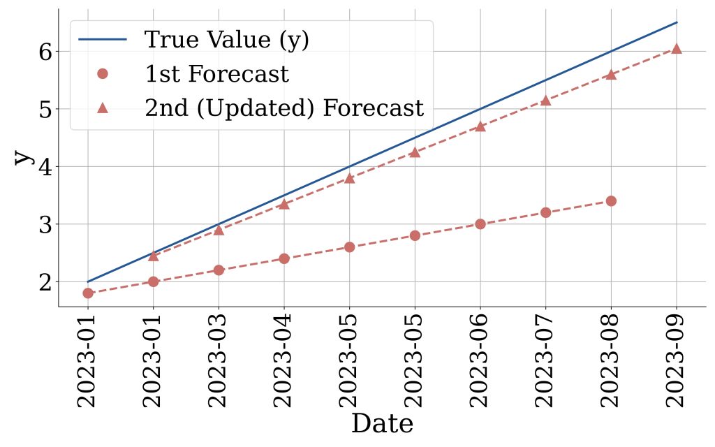
- Zero penalty for improving revisions, shown in Fig. 4a: if a revision moves proportionally closer to the ground truth, landing on the direct path between the truth and the prior forecast, EV = 0.
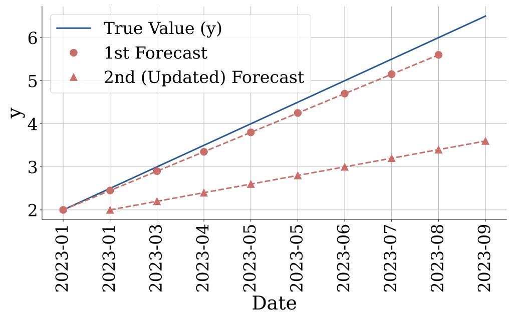
- Maximum penalty for deteriorating revisions, shown in Fig. 4b: if a revision moves the forecast further from the truth, with the old forecast sitting between the truth and the new one, EV equals the full accuracy degradation, the difference in quantile loss between the new forecast and the old one.
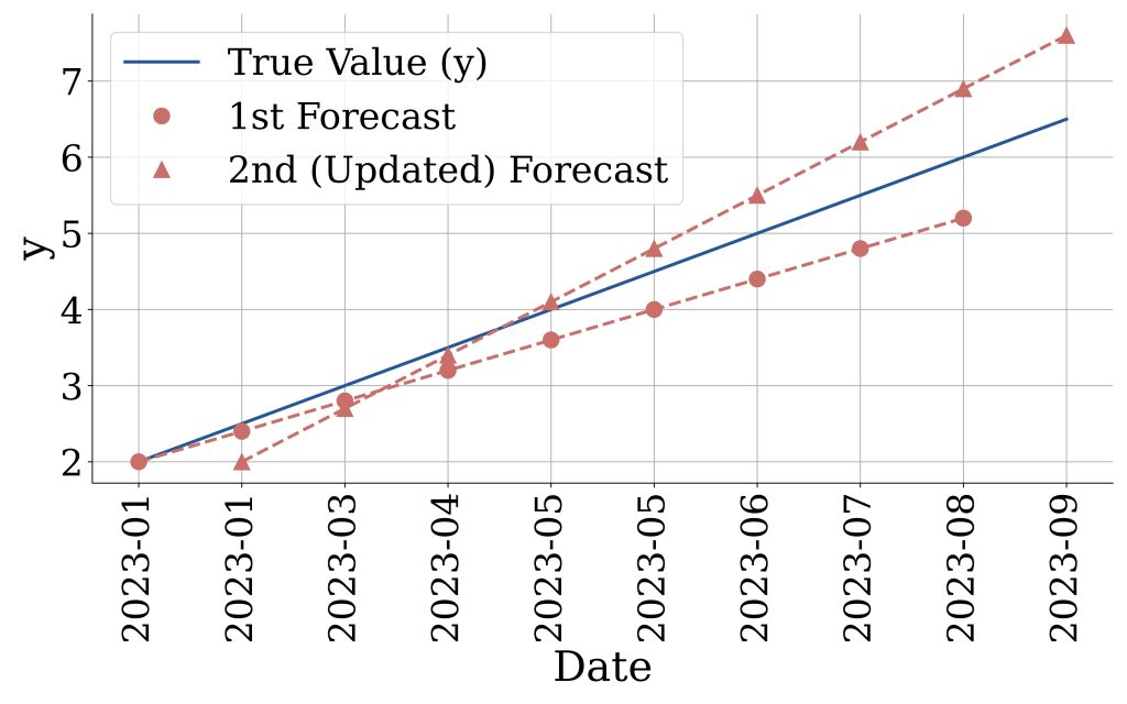
- Overshoot penalty, shown in Fig. 4c: if a revision moves in the right direction but overshoots, with the truth landing between the old and new forecast, EV penalizes only the new forecast's quantile loss against the truth.
 (a) Improving revision
 (b) Deteriorating revision
 (c) Overshooting revision
Fig. 4: Example penalty behavior of the Excess Volatility (EV) metric. EV distinguishes accuracy-improving revisions from accuracy-degrading ones, assigning no penalty when revisions improve accuracy, while asymmetrically penalizing both deteriorating and overshooting revisions according to their impact on accuracy.
One important distinction: sFPC can be computed at prediction time for real-time monitoring, since it doesn't require ground truth. sEV, by contrast, depends on the ground-truth value, so it can only be applied retroactively to assess forecast volatility.
Empirical Results: Volatility Reduction Without Sacrificing Accuracy
The core empirical claim: for forking-sequences models, applying exponential-smoothing ensembling at inference (α = 0.9) reduces forecast volatility (sEV) substantially while maintaining forecast accuracy.
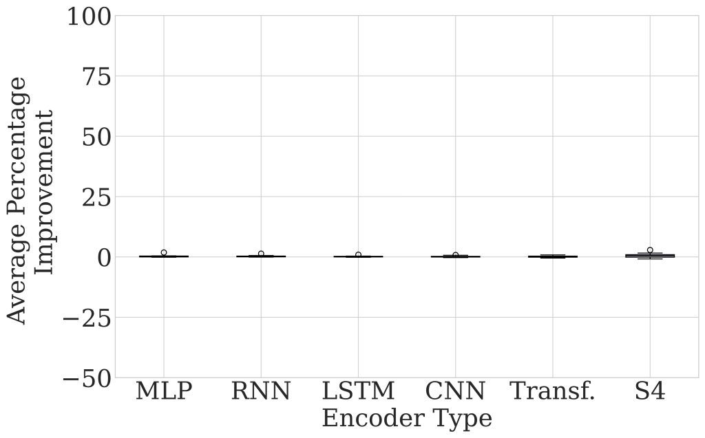
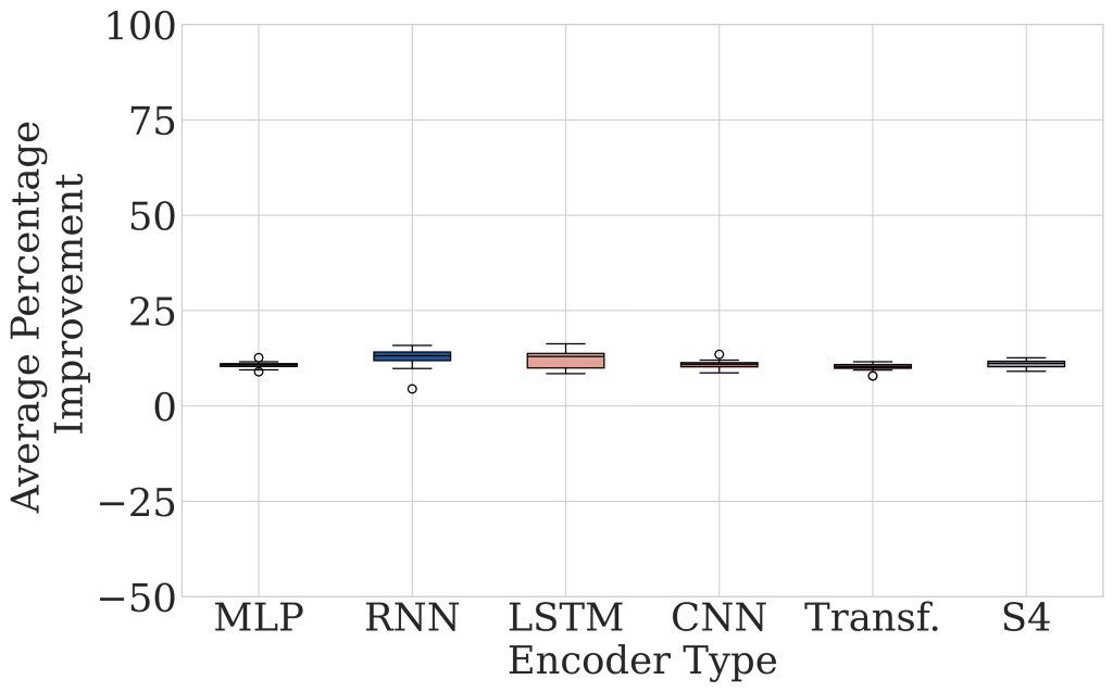
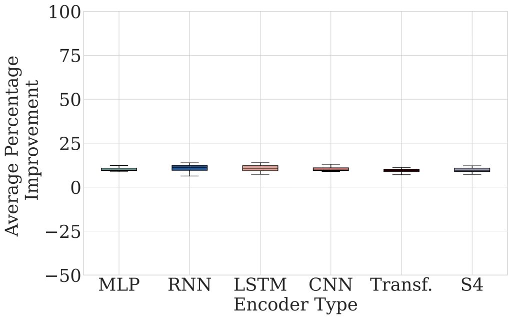
We show that for forking-sequences models, forecast ensembling during inference can reduce forecast volatility compared to forecasts without ensembling for all encoders. Specifically, applying exponential smoothing at inference to models trained with forking-sequences yields median percentage improvements in sEV across datasets of 13.2%, 13.0%, 10.9%, 10.2%, and 11.2% for RNN, LSTM, CNN, Transformer, and StateSpace-based architectures, respectively, while maintaining forecast accuracy (less than 0.1% degradation in sCRPS as shown in Fig. 5).
 (a) sCRPS
 (b) sEV
 (c) sFPC
Fig. 5: Distribution of percentage improvement in (a) sCRPS, (b) sEV, and (c) sFPC metrics across datasets for different encoder types with forking-sequences forecast ensembling compared with no ensembling. Each dataset's metric is averaged over 5 random seed runs. Percentage improvement greater than zero indicates forecast ensembling achieves lower forecast error or volatility.
We include an ablation study across different ensembling strategies (moving average, moving median, cumulative average, exponential smoothing at α = 0.1/0.5/0.9), and find that exponential smoothing with high α (0.9) gives the best trade-off; it weights near-term (more accurate) forecasts more heavily, minimizing the accuracy cost of smoothing out volatility. Lower α values reduce volatility further but at a higher cost to accuracy.
A Bonus: Zero-Shot Volatility Reductions for Pretrained Foundation Models
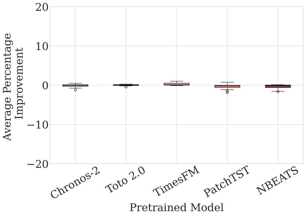
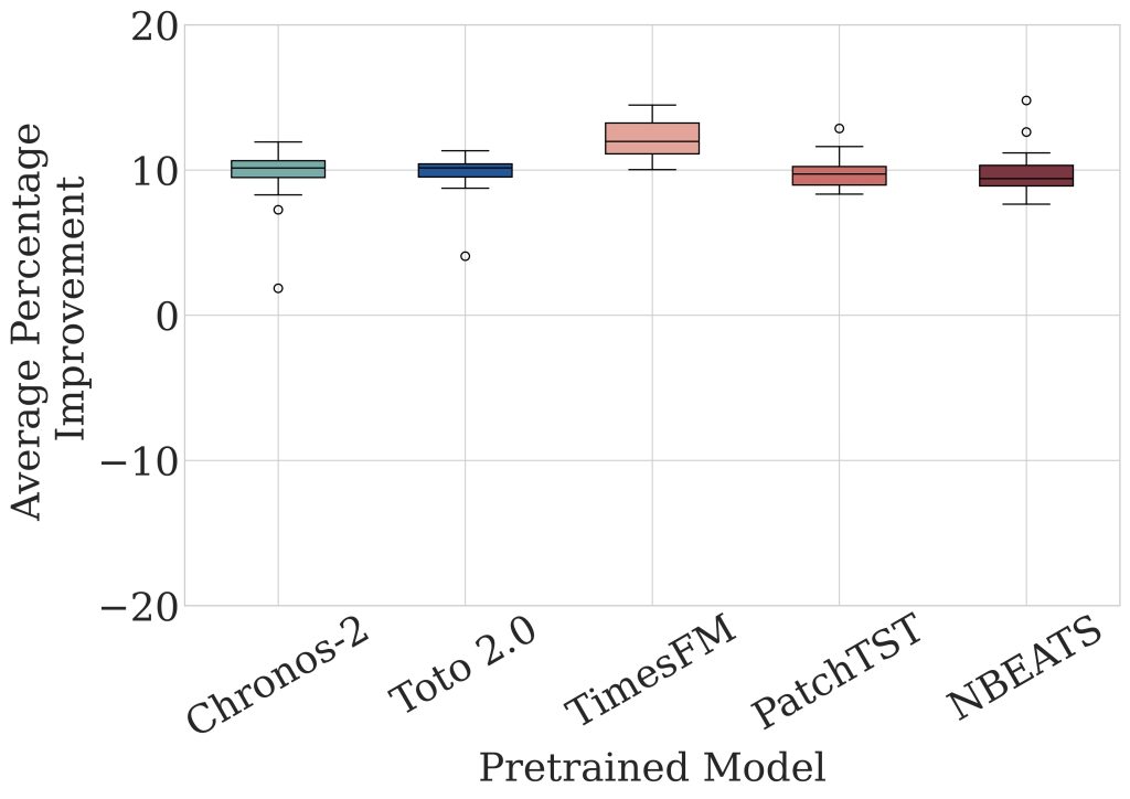
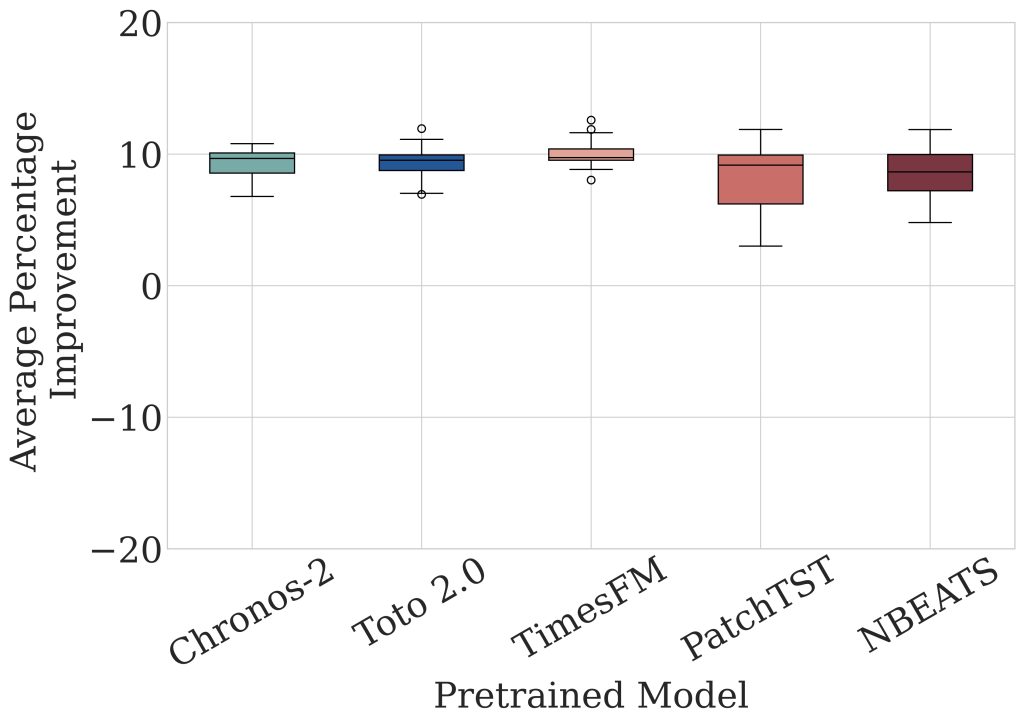
Forecast ensembling benefit isn't limited to models specifically trained with forking-sequences. We can apply forecast ensembling to pretrained models originally trained with window-sampling by collecting forecast revision outputs. We demonstrate this with pretrained Time Series Foundation Models (TSFMs), including Chronos-2, Toto 2.0, TimesFM, and pretrained PatchTST and NBEATS, in a zero-shot setting.
 (a) sCRPS
 (b) sEV
 (c) sFPC
Fig. 6: Distribution of percentage improvement in (a) sCRPS, (b) sEV, and (c) sFPC metrics across datasets for different encoder types with forking-sequences forecast ensembling compared with no ensembling. Percentage improvement greater than zero indicates forecast ensembling achieves lower forecast error or volatility. Forecast ensembling can substantially reduce forecast volatility (sEV, sFPC) while maintaining forecast accuracy (sCRPS), demonstrating its utility as a general-purpose inference technique for models trained with either forking-sequences or window-sampling.
Across the M-series benchmark, this simple technique achieved a median ~10% reduction in forecast volatility, with less than 0.1% degradation in accuracy (sCRPS). In other words: forecast ensembling via forking-sequences-style aggregation is a general-purpose, nearly-free technique that can be used in forecasting pipelines regardless of whether the underlying model was originally trained with forking-sequences.
🔑 Takeaways
1
Forking-sequences' grid structure naturally produces overlapping forecasts across FCDs, enabling near-free ensembling at inference time by reusing already-computed encoder outputs.
2
The new scaled Excess Volatility (sEV) metric distinguishes accuracy-improving revisions from harmful ones — a meaningful improvement over naive percentage-change volatility measures.
3
Ensembling forking-sequences forecasts via exponential smoothing cuts volatility by ~10–13% across encoder architectures without sacrificing accuracy.
4
This benefit extends to zero-shot use with pretrained foundation models like Chronos-2, Toto 2.0, and TimesFM, achieving approximately 10% reduced forecast volatility with <0.1% accuracy cost.
We acknowledge that ensembling can be integrated during both training and inference with forking-sequences, and could be further extended with learnable parameters as explored in [2]. We leave training-time ensembling integration to future work.
Together, Parts I and II aim to build broader awareness of forking-sequences and promote its adoption as a default architectural option in open-source neural forecasting libraries and future research. This work also advocates for greater awareness of volatility metrics as a complement to standard accuracy metrics, encouraging their routine adoption in forecasting evaluation.
References:
[1] Rob J. Hyndman and Anne B. Koehler. Another look at measures of forecast accuracy. International Journal of Forecasting, 22(4):679 – 688, 2006. ISSN 0169-2070.
[2] Carson Eisenach, Yagna Patel, and Dhruv Madeka. MQTransformer: Multi-Horizon Forecasts with Context Dependent and Feedback-Aware Attention. In Maria Florina Balcan and Marina Meila, editors, Submitted to Proceedings of the 38th International Conference on Machine Learning. PMLR. Working Paper version available at arXiv:2009.14799, 8 2021.
